In machine learning many different losses exist.

A loss is a “penalty” score to reduce when training an algorithm on data. It is usually called the objective function to optimize. For an introduction to machine learning and loss functions, you might read Course 0: deep learning! first.

Here we’ll list more losses for the different cases. Knowing each of them will help the datascientists choose the right one for his problem.

The likelihood and the log loss

Classifying means assigning a label to an observation :

Such a function is named a classifier. To create such classifier, we usually create models with parameters to define :

The process of defining the optimal parameters w given past observations X and their known labels Y is named training. The objective of the training is obviously to maximise the likelihood

Since the logarithm is monotonous, it is equivalent to minimize the negative log-likelihood :

The reason for taking the negative of the logarithm of the likelihood are

• it is more convenient to work with the log, because the log-likelihood of statistically independant observation will simply be the sum of the log-likelihood of each observation.

• we usually prefer to write the objective function as a cost function to minimize.

Binomial probabilities - log loss / logistic loss / cross-entropy loss

Binomial means 2 classes, which are usually 0 or 1.

Each class has a probability \(p\) and \(1 - p\) (sums to 1).

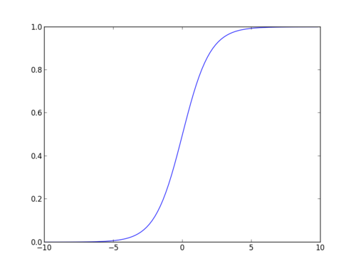
When using a network, we try to get 0 and 1 as values, that’s why we add a sigmoid function or logistic function that saturates as a last layer :

Then, once the estimated probability to get 1 is \(\hat{p}\) (sometimes written \(ŷ\) also), then it is easy to see that the negative log likelihood can be written

which is also the cross-entropy

In information theory, if you try to identify all classes with a code of a length depending of his probability, that is \(- \log q\), where q is your estimated probability, then the expected length in reality (p being the real probability) is given by the cross-entropy.

Note that in natural language processing, we may also speek of perplexity defined by

seen as an indicator of the number of possibilities for the variable to predict, since the perplexity of a uniform k-class random variable would be k.

Last, let’s remind that the combined sigmoid and cross-entropy has a very simple and stable derivative

NB: if you choose that your labels \(y \in \{ \pm 1 \}\), you can write the binary logistic loss

Multinomial probabilities / multi-class classification : multinomial logistic loss / cross entropy loss / log loss

It is a problem where we have k classes or categories, and only one valid for each example.

The target values are still binary but represented as a vector y that will be defined by the following if the example x is of class c :

If \(\{ p_i \}\) is the probability of each class, then it is a multinomial distribution and

The equivalent to the sigmoid function in multi-dimensional space is the softmax function or logistic function or normalized exponential function to produce such a distribution from any input vector z :

The error is also best described by cross-entropy :

Cross-entropy is designed to deal with errors on probabilities. For example, \(\ln(0.01)\) will be a lot stronger error signal than \(\ln(0.1)\) and encourage to resolve errors. In some cases, the logarithm is bounded to avoid extreme punishments.

In information theory, optimizing the log loss means minimizing the description length of y. The information content of a random variable to be in the class being \(- \ln p_i\).

Last, let’s remind that the combined softmax and cross-entropy has a very simple and stable derivative.

Multi-label classification

There is a variant for multi-label classification, in this case multiple \(y_i\) can have a value set to 1.

For example, “car”, “automotible”, “motor vehicule” are three labels that can be applied to a same image of a car. On the image of a truck, you’ll only have “motor vehicule” active for example.

In this case, the softmax function will not apply, we usually add a sigmoïd layer before the cross-entropy layer to ensure stable gradient estimation :

The cross-entropy will look like :

Infogain loss / relative entropy

Many synonym exists : Kullback–Leibler divergence, discrimination information, information divergence, information gain, relative entropy, KLIC, KL divergence.

It measures the difference between two probabilities.

hence in our nomenclature :

The infogain is the difference between the entropy before and the entropy after.

Square error / Sum of squares / Euclidian loss

This time, contrary to previous estimations that were probabilities, when predictions are scalars or metrics, we usually use the square error or euclidian loss which is the L2-norm of the error :

Minimising the squared error is equivalent to predicting the (conditional) mean of y.

Due to the gradient being flat at the extremes for a sigmoid function, we do not use a sigmoid activation with a squared error loss because convergence will be slow if some neurons saturate on the wrong side.

A squared error is often used with a rectified linear unit.

The L2 norm penalizes large errors more strongly and therefore is very sensitive to outliers. To avoid this, we usually use the squared root version :

Absolute value loss / L1 loss

The absolute value loss is the L1-norm of the error :

Minimizing the absolute value loss means predicting the (conditional) median of y. Variants can handle other quantiles. 0/1 loss for classification is a special case.

Note that the L1 norm is not differentiable in 0, and it is possible to use a smooth L1 :

Although the L2 norm is more precise and better in minizing prediction errors, the L1 norm produces sparser solutions, ignore more easily fine details and is less sensitive to outliers. Sparser solutions are good for feature selection in high dimensional spaces, as well for prediction speed.

Hinge loss / Maximum margin

Hinge loss is trying to separate the positive and negative examples \((x,y)\), x being the input, y the target \(\in \{-1, 1 \}\), the loss for a linear model is defined by

The minimization of the loss will only consider examples that infringe the margin, otherwise the gradient will be zero since the max saturates.

In order to minimize the loss,

• positive example will have to output a result superior to 1 : \(w \cdot x > 1\)

• negative example will have to output a result inferior to -1 : \(w \cdot x < - 1\)

The hinge loss is a convex function, easy to minimize. Although it is not differentiable, it’s easy to compute its gradient locally. There exists also a smooth version of the gradient.

Squared hinge loss

It is simply the square of the hinge loss :

One-versus-All Hinge loss

The multi-class version of the hinge loss

where

Crammer and Singer loss

Crammer and Singer defined a multi-class version of the hinge loss :

so that minimizing the loss means to do both :

• maximize the prediction \(w_y \cdot x\) of the correct class

• minimize the predicted value \(w_c \cdot x\) for all other classes c that have the maximal value

until for all these other classes, their predicted values \(w_c \cdot x\) are all below \(w_y \cdot x -1\), the value for the correct class with a margin of 1.

Note that is possible to replace the 1 with a smooth \(\Delta ( y, c)\) value that measures the dissimilarity :

L1 / L2, Frobenius / L2,1 norms

It is frequent to add some regularization terms to the cost function

such as

• the L1-norm, for the LASSO regularization

• the L2-norm or Frobenius norm, for the ridge regularization

• the L2,1 norm, used for discriminative feature selection

Joint embedding

A joint loss is a sum of two losses :

and in the case of multi-modal classification, where data is composed of multiple parts, such as for example images (x1) and texts (x2), we usually use the joint loss with multiple embeddings, which are high dimensional feature spaces :

and a similarity function, such as for example,

In these examples of zero-shot learning where a simple classical multi-class hinge loss was able to train classifiers using precomputed output embedding for each class, a joint embedding loss can train the two embeddings simultanously.

The joint embedding optimization can also be seen as maximizing the log-likelihood for a binomial problem where the output variable is the degree of similarity \(s_{1,2} = [ y_1 == y_2 ]\) and the input variable \(X = (x_1,x_2)\) the combined modalities :

where

Hence, maximizing

In Zero shot learning via joint latent similarity Embedding, Zhang et al. propose an algorithm that iteratively assigns to each example in the dataset an embedding value \((z_1, z_2)\) that maximizes the objective function over all data, then optimizes \(w = ( w_1,w_2,w_3 )\) for this assignment at a very good computational cost.

Connectionist temporal classification loss

This loss function is designed for temporal classification, to have the underlying network concentrate its discriminative capacity and sharpen its classification around spikes.

This loss has been used in audio classification.

We consider sequences x of length T, depending of the sampling interval. The idea is to design a network that is able to predict the correct class as well as blanks during no class is predicted. The underlying network output is enhanced with a blank class, and the output dictionary becomes \(L \cup \{ blank \}\). At each time step or audio frame, the network will predict the class probability \(y_k^t\) and the probability of a path is given by

Nevertheless not every path can be a label : in audio classification, if successive frames are too close, they will correspond to the same phoneme, that’s why the first rule is to reduce successive identical predictions into 1 phoneme if there is no blank between them. Also blanks can be removed.

and the probability of a label in the CTC loss is defined as the sum of the probabilities of all paths reducing to it :

The CTC loss is simply the negative log likelihood of this probability for correct classification

The original paper gives the formulation to compute the derivative of the CTC loss.

You’re all set for choosing the right loss functions.