Course 1: learn to program deep learning in Pytorch, MXnet, CNTK, Tensorflow and Keras!
Here is my course of deep learning in 5 days only!
You might first check Course 0: deep learning! if you have not read it. A great article about cross-entropy and its generalization.
In this article, I’ll go for the introduction to deep learning and programming, coding few functions under deep learning technologies: Pytorch, Keras, Tensorflow, MXNet, CNTK.
Your programming environment
Deep learning demands heavy computations so all deep learning libraries offer the possibility of parallel computing on GPU rather CPU, and distributed computed on multiple GPUs or instances.
The use of specific hardwares such as GPUs requires to install an up-to-date driver in the operating system first.
While OpenCL (not to confuse with OpenGL for graphics or OpenCV for images) is an open standard for scientific GPU programming, the most used GPU library is CUDA, a private library by NVIDIA, to be used on NVIDIA GPUs only.
CUDNN is a second library coming with CUDA providing you with more optimized operators.
Once installed on your system, these libraries will be called by higher level deep learning frameworks, such as Caffe, Tensorflow, MXNet, CNTK, Torch or Pytorch.
The command nvidia-smi enables you to check the status of your GPUs, as with top or ps commands for CPUs.
Most recent GPU architectures are Pascal and Volta architectures. The more memory the GPU has, the better. Operations are usually performed with single precision float16 rather than double precision float32, and on new Volta architectures offer Tensor cores specialized with half precision operations.
One of the main difficulties come from the fact that different deep learning frameworks are not available and tested on all CUDA versions, CUDNN versions, and even OS. CUDA versions are not available for all driver versions and OS as well.
Solutions are:
-
use Docker containers, which limit the choice of the driver version in the host operating system. For the compliant CUDA and CUDNN versions as well as the deep learning frameworks, you install them in the Docker container.
-
or use environment managers such as
condaorvirtualenv. A few commands to know:
#create an environment named pytorch
conda create -n pytorch python=3.4

# activate it
source activate pytorch

# install pytorch in this environment
conda install pytorch

# you are done!
# Run either a python shell
python
# or jupyter notebook
conda install jupyter
jupyter notebook
Jupyter UI proposes to choose the Conda environment inside the notebook.
It is possible to combine CUDA and OpenGL for graphical applications requiring deep learning predictions: the image data is fully processed on GPU.
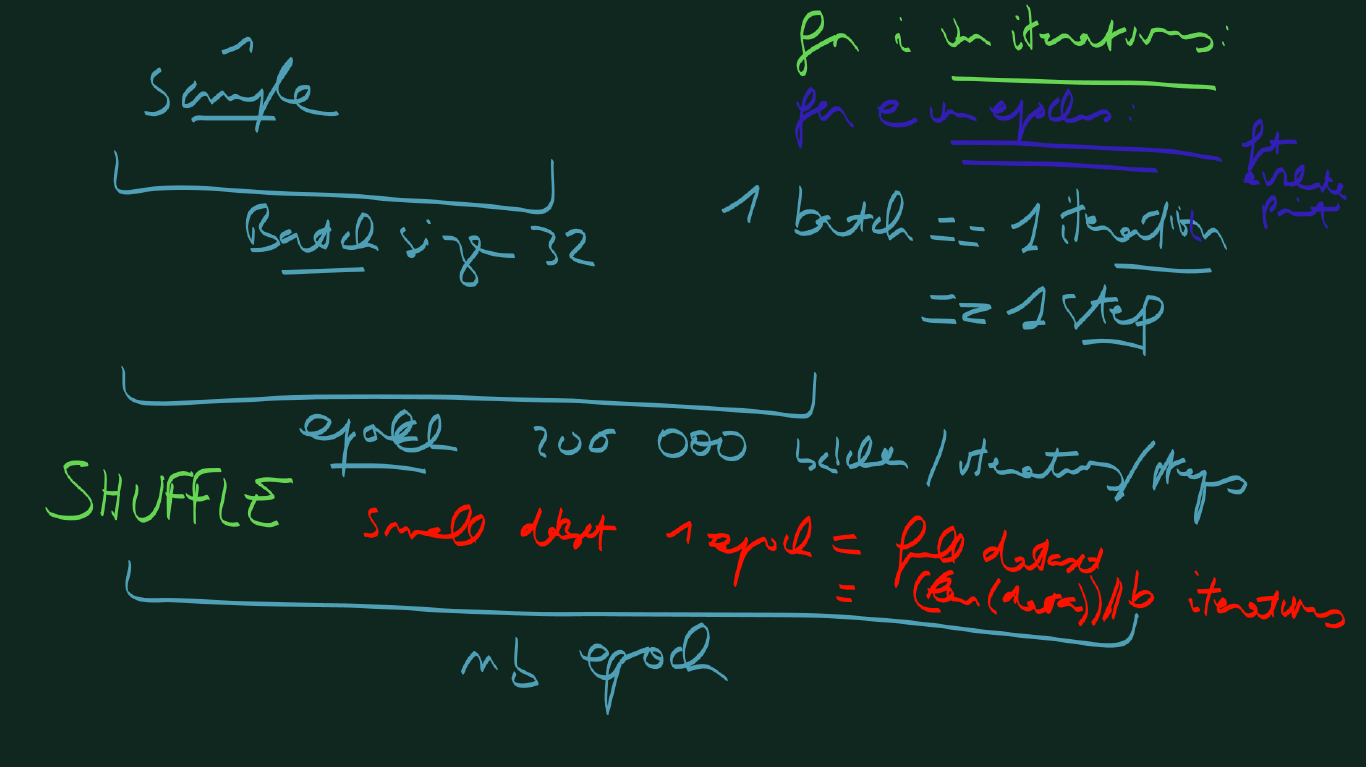
The batch
When applying the update rule, the best is to compute the gradients on the whole dataset but it is too costly. Usually we use a batch of training examples, it is a trade-off that performs better than a single example and is not too long to compute.
The learning rate needs to be adjusted depending on the batch size. The bigger the batch is, the bigger the learning rate can be.
All deep learning programms and frameworks consider the first dimension in your data as the batch size. All other dimensions are the data dimensionality. For an image, it is BxHxWxC, written as a shape (B, H, W, C). After a few layers, the shape of the data will change to (B, h, w, c) : the batch size remains constant, the number of channels usually increases \(c \geq C\) with network depth while the feature map decreases \(h \leq H, w \leq W\) for top layers’ outputs’ shapes.
This format is very common and is called channel last. Some deep learning frameworks work with channel first, such as CNTK, or enables to change the format as in Keras, to (B, C, W, H).
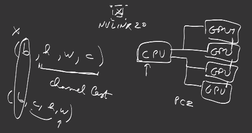
To distribute the training on multiple GPU or instances, the easiest way is to split along the batch dimension, which we call data parallellism, and dispatch the different splits to their respective instance/GPU. The parameter update step requires to synchronize more or less the gradient computations. NVIDIA provides fast multi-gpu collectives in its library NCCL, and fast hardware connections between GPUs with NVLINK2.0.
At the basis of the training is the sample (the example, the datapoint). The batch or minibatch is the training of multiple samples in one iteration or step. An epoch is usually seen as the number of iteration to see the whole training dataset, although in some training programs, for very huge dataset, the epoch is defined as a number of iterations after which the model is evaluated to monitor the training and follow metrics. A shuffle operation of the dataset is required at each epoch.
Training curves and metrics
As we have seen on Course 0, we use a cost function to fit the model to the goal.
So, during training of a model, we usually plot the training loss, and if there is no bug, it is not surprising to see it decreasing as the number of training steps or iterations grows.
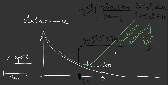
Nevertheless, we usually keep 2 to 10 percent of the training set aside from the training process, which we call the validation dataset and compute the loss on this set as well. Depending if the model has enough capacity or not, the validation loss might increase after a certain step: we call this situation overfitting, where the model has too much learned the training dataset, but does not generalize on unseen examples. To avoid this situation to happen, we monitor the validation metrics and stop the training process when the validation metrics increase, after which the model will perform less.
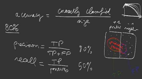
On top of the loss, it is possible to monitor other metrics, such as for example the accuracy. Metrics might not be differentiable, and minimizing the loss might not minimize the metrics. In image classification, a very classical one is the accuracy, that is the ratio of correctly classified examples in the dataset. The opposite is the error rate.
We also usually compute the precision/recall curve: precision defines the number of true positive in the examples predicted as positive by the model (true positives + false positives) while the recall is the number of true positives of the total number of positives (true positives + false negatives). While for some applications, such as document retrieval, we prefer to have higher recall, for some other applications, such as automatic document classification, we prefer to have a high precision for automatically classified documents, and leave ambiguities to human operators.
In order to summarize the quality of the model into one value, one can compute :
-
either the Area Under the Curve (AUC) instead of the full precision/recall curve,
-
or the F1-score, which is \(2 \times \frac{\text{precision} \times \text{recall}}{ \text{precision} + \text{recall} }\)
-
or more generally the \(F_\beta = (1+\beta^2) \times \frac{\text{precision} \times \text{recall}}{ \beta^2 \times \text{precision} + \text{recall} }\)
A library for deep learning
A deep learning library offers the following characteristics :
-
It works very well with Numpy arrays. Arrays are called Tensors. Moreover, operations on Tensors follow lot’s of Numpy conventions.
-
It provides abstract classes, such as Tensors, for parallel computing on GPU rather CPU, and distributed computing on multiple GPUs or instances, since Deep learning demands huge computations.
-
Operators have a ‘backward’ implementation, computing the gradients for you, with respect to the inputs or parameters.
Let’s load Pytorch module into a Python shell, as well as Numpy library, check the Pytorch version is correct and the Cuda library is correctly installed (if you have a GPU only):
import torch
import numpy as np
print(torch.__version__) # 0.4.1
print(torch.cuda.is_available()) # True
1. Numpy compatibility
You can easily check the following commands in Pytorch and Numpy:
| ####### Command ####### | ####### Numpy ####### | ####### Pytorch ####### |
|---|---|---|
| Array conversion | np.array([[1,2]]) | torch.Tensor([[1,2]]) |
| 5x3 matrix, uninitialized | x = np.empty((5,3)) | x = torch.Tensor(5,3) |
| initialized with ones | x = np.ones((5,3)) | x = torch.ones(5,3) |
| initialized with zeros | x = np.zeros((5,3)) | x = torch.zeros(5,3) |
| uniformly randomly initialized matrix | x = np.random.rand(5,3) | x = torch.rand(5, 3) |
| normal randomly initialized matrix | x = np.random.randn(5,3) | x = torch.randn(5, 3) |
| Shape/size | x.shape | x.size |
| Elementwise Addition | +/np.add | +/torch.add |
| In-place multiplication | * | * |
| In-place addition | x+= | x.add_() |
| First column | x[:, 1] | x[:, 1] |
| Matrix multiplication | .matmul() | .mm() |
| Matrix-Vector multiplication | - | .mv() |
| Reshape | .reshape(shape) | .view(size) |
| Transpose | np.transpose(,(1,0)) | torch.transpose(,0,1) |
| Concatenate | np.concatenate([]) | torch.cat([]) |
| Stack | np.stack([], 1) | torch.stack([], 1) |
| Add a dimension | np.expand_dims(, axis) | .unsqueeze(axis) |
| Squeeze a dimension | np.squeeze(, axis) | .squeeze(axis) |
| Range of values | np.arange() | torch.arange() |
| Maximum of the array | np.amax(, axis) | torch.max(, axis) |
| Elementwise max | np.maximum(a,b) | torch.max(a,b) |
.
You can link Numpy array and Torch Tensor, either with
numpy_array = np.ones(5)
torch_array = torch.from_numpy(numpy_array)
or
torch_array = torch.ones(5)
numpy_array = torch_array.numpy()
which will keep the pointers to the original values:
numpy_array+= 1
print(torch_array) # tensor([2., 2., 2., 2., 2.])
torch_array.add_(1)
print(numpy_array) # [3. 3. 3. 3. 3.]
Exercise: find the equivalent operations under Tensorflow, Keras, CNTK, MXNET
Solution: tensorflow, keras, mxnet, cntk
2. GPU computing
It is possible to transfer tensors between devices, ie RAM memory and each GPUs’ memory:
a = torch.ones(5,) # tensor([1., 1., 1., 1., 1.])
b = torch.ones(5,)
a_ = a.cuda() # tensor([1., 1., 1., 1., 1.], device='cuda:0')
b_ = b.cuda()
x = a_ + b_ # tensor([2., 2., 2., 2., 2.], device='cuda:0')
y = x + 1 # tensor([3., 3., 3., 3., 3.], device='cuda:0')
z = y.cuda(1) # tensor([3., 3., 3., 3., 3.], device='cuda:1')
t = z.cpu() # tensor([3., 3., 3., 3., 3.])
but keep in mind that synchronization is lost (contrary to Numpy Arrays and Torch Tensors, it cannot be pointers since the values are not anymore on the same device):
a.add_(1)
print(a_) # tensor([1., 1., 1., 1., 1.], device='cuda:0')
Tensors behave as classical programming non-reference variables and their content is copied from device to the other. This way, you decide when to transfer the data.
Contrary to other frameworks, Pytorch does not require to build a graph of operators and execute the graph on a device. Pytorch programming is as normal Python programming.
3. Automatic differentiation
To compute the gradient automatically, you need to wrap the tensors in Variable objects:
from torch.autograd import Variable
x = Variable(torch.ones(1)+1, requires_grad=True)
print(x.data)
#tensor([2.])
print(x.grad)
# None
print(x.grad_fn)
# None
The Variable contains the original data in the data attribute. The API for Tensors is also available for Variables.
When you add an operation such as for example the square operator, the newly created Variable is populated with the result in the data attribute as well as an history grad_fn function :
y = x ** 2
print(y.data)
# tensor([4.])
print(y.grad)
# None
print(y.grad_fn)
# <PowBackward0 object at 0x7ffaf1ae0160>
The grad_fn Function contains the history or the link to x, which enables to compute the derivative thanks to the Variable’s backward() method:
y.backward()
print(x.data)
# tensor([2.])
print(x.grad)
# tensor([4.])
The gradient of the cost y with respect to the input x is placed in x.grad and since \(\frac{\partial x^2}{\partial x} = 2 x\), its value is 4 at x=2.
Exercise: with Torch, compute the gradient of \(z = 3 x + 2 y\) with respect to x=5 and y=2.
Calling y.backward() a second time will lead to a RunTime Error. In order to accumulate the gradients into x.grad, you need to set retain_graph=True during the first backward call.
Let’s confirm this in a case where the input is multi-dimensional and reduced into a scalar with a sum operator:
x = Variable(torch.ones(2), requires_grad=True)
y = x.sum()
y.backward(retain_graph=True)
print(x.grad)
# tensor([1., 1.])
y.backward()
print(x.grad)
# tensor([2., 2.])
y.backward()
print(x.grad)
# tensor([3., 3.])
Since \(\frac{\partial}{\partial x_1} (x_1 + x_2) = 1\) and \(\frac{\partial}{\partial x_2} (x_1 + x_2) = 1\), the x.grad tensor is populated with ones.
Applying the backward() method multiple times accumulates the gradients.
It is also possible to apply the backward() method on something else than a cost (scalar), for example on a layer or operation with a multi-dimensional output, as in the middle of a neural network, but in this case, you need to provide as argument to the backward() method \(\Big( \nabla_{I_{t+1}} \text{cost} \Big)\), the gradient of the cost with respect to the output of the current operator/layer (which is written here as the input of the operator/layer above), which will be multiplied by \(\Big( \nabla_{\theta_t} L_t \Big)\), the gradient of the current operator/layer’s output with respect to its parameters, in order to produce the gradient of the cost with respect to the current layer’s parameters:
as given by the chaining rule seen in Course 0.
x = Variable(torch.ones(2), requires_grad=True)
y = x ** 2
print(y.data)
# tensor([1., 1.])
y.backward(torch.tensor([-1., 1.]))
print(x.grad)
# tensor([-2.,  2.])
The gradient of the final cost with respect to the output of the current operator/layer indicates how to combine the derivatives of different output values in the current layer in the production of a derivative with respect to each parameter.
As Pytorch does not require to introduce complex graph operators as in other technologies (switches, comparisons, dependency controls, scans/loops… ), it enables you to program as normally, and gradients are well propagated through your Python code:
x = Variable(torch.ones(1) +1, requires_grad=True)
y = x
while y < 10:
  y = y**2
print(y.data)
# tensor([16.])
y.backward()
print(x.grad)
# tensor([32.])
which is fantastic. In this case, \(y\vert_{x=2} = ( x^2 )^2 = x^4\) and \(\frac{\partial y}{\partial x} \big\vert_{x=2} = 4 x^3 = 32\).
Note that gradients are computed by retropropagation until a Variable has no graph_fn (an input Variable set by the user) or a Variable with requires_grad set to False, which helps save computations.
Exercise: compute the derivative with Keras, Tensorflow, CNTK, MXNet
Training loop
Let’s take back our Course 0’s perceptron and implement its training directly with Pytorch tensors and operators, without other packages. Let’s consider the input is 20 dimensional, and the number of outputs for each dense layer is 32.
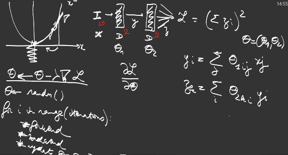
Pytorch only requires to implement the forward pass of our perceptron. Each Dense layer is composed of two learnable parameters or weights:
theta1 =  Variable(torch.randn(32,20) *0.1,requires_grad = True)
bias1 = Variable(torch.randn(32)*0.1,requires_grad = True)
theta2 = Variable(torch.randn(32,32)*0.1,requires_grad = True)
bias2 = Variable(torch.randn(32)*0.1,requires_grad = True)

def forward(x):
    # affine operation of the first Dense layer
    y = theta1.mv(x) + bias1
    # ReLu activation
    y = torch.max(y, Variable(torch.Tensor([0])))
    # affine operation of the second Dense layer
    return theta2.mv(y) + bias2
As first loss function, let’s use the square of the sum of the outputs. We can take whatever we want, as soon as it returns a scalar value to minimize:
def cost(z):
    return (torch.sum(z)) ** 2
A training loop iterates over a dataset of training examples and each iteration consists in
-
a forward pass : propagate the input values through layers from bottom to top, until the cost/loss
-
a backward pass : propagate the gradients from top to bottom and into each of the parameters
-
apply the parameter update rule \(\theta \leftarrow \theta - \lambda \nabla_{\theta_L} \text{cost}\) for each layer L
Let’s train this network on random inputs, one sample at a time:
for i in range(1000):
    lr = 0.001 * (.1 ** ( max(i - 500 , 0) // 100))

    x = Variable(torch.randn(20), requires_grad=False)
    z = forward(x)
    c = cost(z)
    print("cost {} - learning rate {}".format(c.data.item(), lr))

    # compute the gradients
    c.backward()

    # apply the gradients
    theta1.data = theta1.data - lr * theta1.grad.data
    bias1.data = bias1.data - lr * bias1.grad.data
    theta2.data = theta2.data - lr * theta2.grad.data
    bias2.data = bias2.data - lr * bias2.grad.data

    # clear the grad
    theta1.grad.zero_()
    bias1.grad.zero_()
    theta2.grad.zero_()
    bias2.grad.zero_()
Exercise: check the norm of the parameters at every iteration.
In a classification task,
-
training is usually performed on batch of samples, instead of 1 sample, at each iteration, to get a faster training, but also to reduce the cost of the transfer of data when the data is moved to GPU
-
the model is required to output a number of values equal to the number of classes, normalized by softmax activation
-
the loss is the cross-entropy
as we have seen in Course 0.
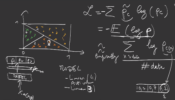
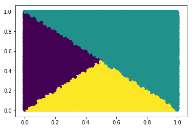
Let us consider a toy data, in which the label of a sample depends on its position in 2D, with 3 labels corresponding to 3 zones:
The dataset creation or preprocessing is usually performed with Numpy:
import matplotlib.pyplot as plt
dataset_size = 200000
x = np.random.rand(dataset_size, 2)
labels = np.zeros(dataset_size)
labels[x[:, 0] > x[:,1]] = 2
labels[x[:,1] + x[:, 0] > 1] = 1
plt.scatter(x[:,0], x[:,1], c=labels )
plt.show()
Let’s convert the Numpy arrays to Torch Tensors:
X = torch.from_numpy(x).type(torch.FloatTensor)
Y = torch.from_numpy(labels).type(torch.LongTensor)
The input is defined by a position, ie a vector of dimension 2 for each sample, leading to a Tensor of size (B, 2), where B is the batch size.
Let’s choose as hidden dimension (number of outputs of first layer/ inputs of second layer) 12:
theta1 =  Variable(torch.randn(2, 12) *0.01,requires_grad = True)
bias1 = Variable(torch.randn(12)*0.01,requires_grad = True)
theta2 = Variable(torch.randn(12, 3)*0.01,requires_grad = True)
bias2 = Variable(torch.randn(3)*0.01,requires_grad = True)

def forward(x):
    y = x.mm(theta1) + bias1 # (B, 2) x (2, 12) + (B, 12) => (B, 12)
    y = torch.max(y, Variable(torch.Tensor([0])))
    y = y.mm(theta2) + bias2 # (B, 12) x (12, 3) + (B, 3) => (B, 3)
    return y

def softmax(z):
    e = torch.exp(z)
    s = torch.sum(e, 1, keepdim = True)
    return e / s

def crossentropy(s, l):
    v = torch.gather(s, 1, torch.unsqueeze(l,-1))
    v = torch.log(v)
    return -torch.mean(v)
For more efficiency, let’s train 20 samples at each step, hence a batch size of 20:
batch_size = 20
for i in range(min(dataset_size, 100000) // batch_size ):
    lr = 0.5 * (.1 ** ( max(i - 100 , 0) // 1000))

    batch = X[batch_size*i:batch_size*(i+1)] # size (batchsize, 2)
    z = forward(Variable(batch, requires_grad=False))
    z = softmax(z)
    loss = crossentropy(z, Variable(Y[batch_size*i:batch_size*(i+1)]))
    print("iter {} - cost {} - learning rate {}".format(i, loss.data.item(), lr))

    # compute the gradients
    loss.backward()

    # apply the gradients
    theta1.data.sub_( lr * theta1.grad.data )
    bias1.data.sub_( lr * bias1.grad.data)
    theta2.data.sub_( lr * theta2.grad.data )
    bias2.data.sub_( lr * bias2.grad.data )

    # clear the grad
    theta1.grad.zero_()
    bias1.grad.zero_()
    theta2.grad.zero_()
    bias2.grad.zero_()
# iter 4999 - cost 0.07717917114496231 - learning rate 5.000000000000001e-05
The network converges.
When loss.backward() is called, the derivatives are propagated through all Variables in the graph, and their .grad attribute accumulated with the gradient (except those with requires_grad set to False):
print(loss.grad_fn)  # NegBackward
print(loss.grad_fn.next_functions[0][0])  # MeanBackward1
print(loss.grad_fn.next_functions[0][0].next_functions[0][0])  # LogBackward
print(loss.grad_fn.next_functions[0][0].next_functions[0][0].next_functions[0][0])  # GatherBackward
To check everything is fine, one might compute the accuracy, a classical metric for classification problems:
accuracy = 0
nb = 10000
for i in range(min(dataset_size, nb)):
    z = forward(Variable(X[i:i+1], requires_grad=False))
    p = softmax(z)
    l = torch.max(p, -1)[1]
    if l.data.numpy()[0] == labels[i]:
        accuracy += 1

print("accuracy {}%".format(round(accuracy / min(dataset_size, nb) * 100,2)))
# accuracy 99.46%
Exercise: compute precision, recall, and AUC.
Note that convergence is strongly influenced
-
by the art of choosing the learning rate
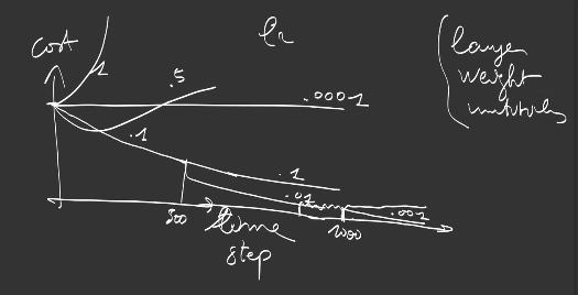
-
by the art of choosing the right layer initialization: a small variance, with positive and negative values to dissociate the neural outputs (neurons that fire together wire together) helps. In fact, we’ll see in the next section Pytorch packages that provide a correct implementation of the variance choice given the number of input and output connections:


To improve the results, it is possible to train multiple times the network from scratch, and average the predictions coming from the ensemble of trained networks.
Note also that, if there is a backward function for every operation, there is no forward function: evaluation is performed when the operator is applied to the variable as in a classical program. It is up to you to create your own forward function as in a classical program. The backward function works as a kind of history of the operations in order to retropropagate the gradient. So, it is very different from the concept of “graph of operators”.
Exercise: program a training loop with Keras, Tensorflow, CNTK, MXNet
Solution: cntk training, mxnet training, keras training, tensorflow training
Pytorch and MXNet work about the same. In MXNet, use attach_grad() on the NDarray with respect to which you’d like to compute the gradient of the cost, and start recording the history of operations with with mx.autograd.record(), then you can use directly backward(). No wrapping in a Variable object as in Pytorch.
In CNTK, Tensorflow and Keras, you build a graph, so you do not get instantly the result of your operation, for example an addition does not give a result but an object that will evaluated in a session on a device by feeding data into the inputs.
- in CNTK, the
Parameterandinput_variableare subclasses of the Variable class so you do not need to wrap them into a Variable object as in Pytorch, but since you build a graph, so you have to callevalorgradmethods on any element of the graph with input values to evaluate them. - Tensorflow is the most complex, but leaves lot’s of freedom. You need to instantiate a session on the device yourself and call the initialization of your variables in the session. The gradient as well as the assignation of values are available operators so that everything can be designed in the graph, but the benefits are extremely small.
- Keras is an abstraction over Tensorflow and CNTK, so you retrieve the points discussed above in the implementation.
Tensorflow has an eager mode option, which enables to get the results of the operator instantly as in Pytorch and MXNet.
Modules
A module is an object that encapsulates learnable parameters and is specifically suited to design deep learning neural networks.
A layer is the smallest module, it has weights and a forward function.:

The composition of multiple modules builds a new module:
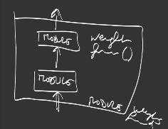
that can be reused at multiple places in the network architecture.
The organization into modules helps interoperability and reuse of modules into a deep neural network definition.
Then, calling the forward or backward propogations, transfering the module to GPU, saving or loading weights, is applied to all submodules without extra code.
Let’s rewrite the previous model as a module, an interface provided by the torch.nn module package, and compose it with prebuilt submodules from the torch.nn.function package:
import torch.nn as nn
import torch.nn.functional as F

class SimpleNetTest(nn.Module):

    def __init__(self):
        super(SimpleNetTest, self).__init__()
        self.lin1 = nn.Linear(2, 12)
        self.lin2 = nn.Linear(12, 3)

    def forward(self, input):
        x = F.relu(self.lin1(input))
        x = self.lin2(x)
        return x

net = SimpleNetTest()
print(net)
# SimpleNetTest(
#   (lin1): Linear(in_features=2, out_features=12, bias=True)
#   (lin2): Linear(in_features=12, out_features=3, bias=True)
# )
The learnable parameters are returned by net.parameters():
params = list(net.parameters())
print(params)
# [Parameter containing:
# tensor([[ 0.5115, -0.1418],
#         [-0.5533, -0.1273],
#         [-0.2584, -0.0393],
#         [-0.6614, -0.3380],
#         [-0.1831,  0.4581],
#         [ 0.3085, -0.6811],
#         [-0.4236, -0.6968],
#         [ 0.2943, -0.2573],
#         [ 0.4532, -0.3313],
#         [ 0.0415, -0.6035],
#         [ 0.0736, -0.0780],
#         [ 0.3948,  0.4727]], requires_grad=True), Parameter containing:
# tensor([ 0.3995,  0.2957,  0.4611, -0.6316, -0.4317,  0.3888, -0.2252,  0.2357,
#          0.0351, -0.0223, -0.2179, -0.0943], requires_grad=True), Parameter containing:
# tensor([[-0.1178,  0.0759,  0.2238, -0.1543,  0.2471,  0.2617,  0.0897, -0.1238,
#          -0.2371,  0.2220, -0.2427, -0.0141],
#         [ 0.2623,  0.2131,  0.0291, -0.1194, -0.1685, -0.1901, -0.0905,  0.1825,
#          -0.0384,  0.2694,  0.0682, -0.0157],
#         [ 0.2674,  0.0229, -0.0429,  0.1274,  0.1928,  0.1575,  0.2514, -0.1529,
#          -0.0460,  0.0187, -0.1481, -0.1473]], requires_grad=True), Parameter containing:
# tensor([-0.2622,  0.0747, -0.2832], requires_grad=True)]
In place of our previous forward(batch) function, we simply apply the batch to the module with net(batch) and loop over the parameters to update them:
batch_size = 20
for i in range(min(dataset_size, 100000) // batch_size ):
    lr = 0.5 * (.1 ** ( max(i - 100 , 0) // 1000))

    batch = X[batch_size*i:batch_size*(i+1)] # size (batchsize, 2)
    z = net(Variable(batch, requires_grad=False))
    z = softmax(z)
    loss = crossentropy(z, Variable(Y[batch_size*i:batch_size*(i+1)]))
    print("iter {} - cost {} - learning rate {}".format(i, loss.data.item(), lr))

    # compute the gradients
    loss.backward()

    # apply the gradients
    for param in net.parameters():
        param.data.sub_( lr * param.grad.data )
        param.grad.zero_()
For the same training on GPU, let’s move our datasets as well the module to GPU:
X = X.cuda()
Y = Y.cuda()
net.cuda()
params = list(net.parameters())
print(params)
# [Parameter containing:
# tensor([[ 2.9374, -2.9921],
#         [-1.8221, -0.3139],
#         [-2.7522, -0.8614],
#         [-0.6614, -0.3380],
#         [-0.1840,  0.4384],
#         [-1.9955, -3.9197],
#         [-0.4236, -0.6968],
#         [ 2.0039,  0.7968],
#         [ 2.5727, -3.4312],
#         [ 0.0331, -0.6036],
#         [ 0.0736, -0.0780],
#         [ 3.9596,  5.2725]], device='cuda:0', requires_grad=True), Parameter containing:
# tensor([ 0.2908,  1.7123,  2.7156, -0.6316, -0.4515,  3.9756, -0.2252, -0.6254,
#          0.6207, -0.0313, -0.2179, -3.2287],
#        device='cuda:0', requires_grad=True), Parameter containing:
# tensor([[-2.8967,  1.5755,  2.2599, -0.1543,  0.2469,  0.7531,  0.0897, -1.1861,
#          -3.3350,  0.2220, -0.2427, -2.1395],
#         [ 2.1709, -0.9695, -1.7979, -0.1194, -0.1682, -3.0841, -0.0905,  1.1191,
#           1.7238,  0.2693,  0.0682,  4.0227],
#         [ 1.1377, -0.2940, -0.2520,  0.1274,  0.1927,  2.5601,  0.2514, -0.0273,
#           1.2897,  0.0188, -0.1481, -2.0602]],
#        device='cuda:0', requires_grad=True), Parameter containing:
# tensor([ 0.7422, -0.9477, -0.2653], device='cuda:0', requires_grad=True)]
All the parameters appear on the first GPU (cuda:0). Note that we transfered the full dataset to the GPU, while in most applications, it is not possible since the memory of the GPU is limited, we only transfer the batch at each iteration.
When the GPU has been used for training, it is a good practice to use it for inference on the test data as well, so we need to rewrite it to train batches of samples rather than samples indiviually:
accuracy = 0
nb = 1000
for i in range(min(dataset_size, nb)):
    z = net(Variable(X[i:i+1], requires_grad=False))
    l = torch.max(z, -1)[1]
    if l.data.cpu().numpy()[0] == Y[i]:
        accuracy += 1

print("accuracy {}%".format(round(accuracy / min(dataset_size, nb) * 100, 2)))
# accuracy 99.2
Exercise: program the training loop with packages in Keras, Tensorflow, CNTK, MXNet
Solution: cntk training, cntk further packaging, keras training, keras further packaging …
Packages
Packages help you reuse common functions for deep learning. We already introduced the torch.nn package containing the module interface as well as prebuilt modules.
Let us rewrite the training loop using the torch.optim package (zeroing gradients + applying the gradients with an update rule), plot the training curves (loss,…) and try different update rules/optimizers.
criterion = nn.CrossEntropyLoss()

import torch.optim as optim
optimizer = optim.SGD(net.parameters(), lr=0.1, momentum=0.9)
The optimizer provides a method zero_grad() to clear the previous gradient values and a step() method to apply the update rule to the parameters:
loss_curve = list()
batch_size = 500
for i in range(min(dataset_size, 1000000) // batch_size ):
batch = X[batch_size*i:batch_size*(i+1)]
batch = Variable(batch, requires_grad=False)
batchLabel = Variable(Y[batch_size*i:batch_size*(i+1)])
# zero the parameter gradients
optimizer.zero_grad()
# forward
outputs = net(batch)
loss = criterion(outputs, batchLabel)
# backward
loss.backward()
# update network parameters
optimizer.step()
# print("iter {} - cost {}".format(i, loss.data.item()))
loss_curve.append(loss.data.item())
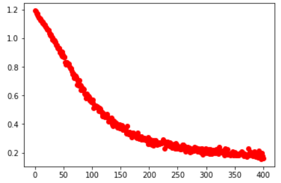
print("final cost {}".format(round(loss.data.item(), 2)))
# final cost 0.04
Let’s plot the training loss:
plt.plot(range(1, len(loss_curve)+1), loss_curve, 'ro')
To compute the accuracy, we can also forward the full dataset and use efficient matrix operations on the final tensors, removing the for loop:
accuracy = 0
z = net(Variable(X, requires_grad=False))
l = torch.max(z, 1)[1]
ll = Variable(Y)
accuracy = int(torch.sum(torch.eq(l, ll).type(torch.cuda.LongTensor)))
print("accuracy {}%".format(round(accuracy / dataset_size * 100,2)))
# accuracy 96.73%
Exercise: try various optimizers and learning rates
optimizer = torch.optim.Adam(net.parameters())
optimizer = torch.optim.Adadelta(net.parameters())
and confirm that Adadelta achieves best accuracy: 99.62%.
Exercise: replace your functions with package functions in MXNet, Keras, Tensorflow, CNTK
Well done!
Now let’s go to next course: Course 2: building deep learning networks!