In this post, I’ll give some explanations about Embedding Symbolic Knowledge into Deep Networks paper (LENSR) and their code for someone interested in the deep understanding of the implementation, not a global overview.

In particular, I’ll answer the following questions:

1/ what are the features X of leaf nodes in the symbolic knowledge embedder ?

2/ How is computed the embedding of the formula ?

3/ How do we link formula satisfaction and model predictions during training ?

And many more frequenlty asked questions.

The goal and datasets

The goal is to use logical rules based on prior knowledge in the training of neural networks.

The idea of the paper is to use Graph Convolutional Networks (GCN) to represent logical formulas with an embedding vector, and to use these representations as a new logical loss, either to predict if an assignment of variables will satisfy a logic, or to train a neural network’s outputs to satisfy a logic.

The evaluation of the representations are performed on 2 datasets:

• a synthetic dataset of logical formulas, to predict if an assignment will satisfy the formulas. Complexity of the formulas depends on the number of variables and the depth. Logic formulas are randomly generated (uniformly sampled propositions and operators) for the synthetic experiments.

• the Visual Relationship Detection (VRD) dataset with its original images from Scene Graph dataset.

The dataset is composed of 100 object classes (objects.json):

'person', 'sky', 'building', 'truck', 'bus', 'table', 'shirt', 'chair', 'car', 'train', 'glasses', 'tree', 'boat', 'hat', 'trees', 'grass', 'pants', 'road', 'motorcycle', 'jacket', 'monitor', 'wheel', 'umbrella', 'plate', 'bike', 'clock', 'bag', 'shoe', 'laptop', 'desk', 'cabinet', 'counter', 'bench', 'shoes', 'tower', 'bottle', 'helmet', 'stove', 'lamp', 'coat', 'bed', 'dog', 'mountain', 'horse', 'plane', 'roof', 'skateboard', 'traffic light', 'bush', 'phone', 'airplane', 'sofa', 'cup', 'sink', 'shelf', 'box', 'van', 'hand', 'shorts', 'post', 'jeans', 'cat', 'sunglasses', 'bowl', 'computer', 'pillow', 'pizza', 'basket', 'elephant', 'kite', 'sand', 'keyboard', 'plant', 'can', 'vase', 'refrigerator', 'cart', 'skis', 'pot', 'surfboard', 'paper', 'mouse', 'trash can', 'cone', 'camera', 'ball', 'bear', 'giraffe', 'tie', 'luggage', 'faucet', 'hydrant', 'snowboard', 'oven', 'engine', 'watch', 'face', 'street', 'ramp', 'suitcase'

70 predicates (predicates.json)

'on', 'wear', 'has', 'next to', 'sleep next to', 'sit next to', 'stand next to', 'park next', 'walk next to', 'above', 'behind', 'stand behind', 'sit behind', 'park behind', 'in the front of', 'under', 'stand under', 'sit under', 'near', 'walk to', 'walk', 'walk past', 'in', 'below', 'beside', 'walk beside', 'over', 'hold', 'by', 'beneath', 'with', 'on the top of', 'on the left of', 'on the right of', 'sit on', 'ride', 'carry', 'look', 'stand on', 'use', 'at', 'attach to', 'cover', 'touch', 'watch', 'against', 'inside', 'adjacent to', 'across', 'contain', 'drive', 'drive on', 'taller than', 'eat', 'park on', 'lying on', 'pull', 'talk', 'lean on', 'fly', 'face', 'play with', 'sleep on', 'outside of', 'rest on', 'follow', 'hit', 'feed', 'kick', 'skate on'

and the files annotations_train.json and annotations_test.json, dictionaries containing for each file a list of annotations inthe JSON format

{
  'predicate': 0,
  'object': {'category': 0, 'bbox': [318, 1019, 316, 767]},
  'subject': {'category': 13, 'bbox': [330, 473, 501, 724]}
}

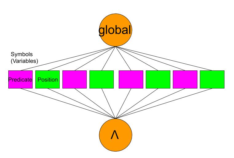
From this training dataset, logical formulas are extracted via rule learning to constrain each relation predicate with all possible relation position between objects. The goal here is to have a neural network prediction of a relation between objects to satisfy the constrains given by the position relation of object bounding boxes.

The dataset is scanned to search for all position relations possible for each relation [predicate, subject, object], among one of 10 possible exclusive names:

'_out', '_in', '_o_left', '_o_right', '_o_up', '_o_down', '_n_left','_n_right', '_n_up', '_n_down'

and build the imply clause \(\text{predicate} \rightarrow \lor \left( \lor \text{position} \right)\) for each predicate.

On top of that, for each subject-object pairs, the equivalent reverse position relation clause is added:

[['_out', '_in'], ['_o_left', '_o_right'], ['_o_up', '_o_down'],['_n_left', '_n_right'], ['_n_up', '_n_down']]

When a sample (image, subject, object) is processed:

• only clauses that apply to two objects available in image are kept,

• the assumption, i.e. the position relation that hold in the current sample, is added as a clause composed of one position variable

For CNF conversion, IDs of relation variables that are kept are remapped to a range of values from 1 to N, a requirement from PySat package.

Logical Graph Forms

Logical formulas are in the general form when arbitrary, but some can be compiled into other simplified graph forms, with some of them with appealing or simplifying characteristics (satisfiability, determinism, decomposability, polytime satisfiabily, polytime counting…).

The Conjunctive Normal Form (CNF)

The CNF is a conjunction (AND) of clauses, where a clause is a disjunction (OR) of literals. A literal is a propositional variable / predicate symbol, possibly preceded by a negation (NOT).

• In the case of the VRD dataset, formula can be directly written in the CNF form. A clause is an imply statement: “Person X wears glasses” implies “glasses are IN Person X” and an imply statement \(P \rightarrow Q\) can be written in the form of a disjunction \(\neg P \lor Q\).

• In the case of the synthetic dataset, the conversion of arbitrary formulas is performed with sympy.logic.to_cnf function from the Sympy package.

The result is saved into DIMACS format.

The decision-Deterministic Decomposable Negation Normal Form (d-DNNF)

The d-DNNF satisfies two properties:

• determinism, requiring operands of an OR to be mutually inconsistent

• decomposability, requiring operands of an AND to be mutually disjoint variables

Conversion from CNF form in DIMACS format to d-DNNF is performed with c2d_linux command (in model.Misc.Formula.dimacs_to_cnf) of the C2D compiler from UCLA.

Graph embedding

Graph Convolution Networks

A stack of multiple Graph Convolution Networks (GCN) is applied to all nodes of a graph of any form. The output of the stack is NxD, where N is the number of graph nodes, and D=100 the dimension of the last layer.

In order to output a global representation of a graph of dimension (D,), a global node is added to the graph, with type global, and linked to all other nodes in the graph: the embedding of this node of dimension D is taken as the graph embedding.

The graph definition, input to GCN, is defined by 2 text files:

• a ‘.var’ file, listing all nodes with their ID, features and label
• an ‘.rel’ file, listing all edges between nodes

In the case of CNF, d-DNNF or assignments, the features for a negated literal ‘-i’ is assigned with the negative vector of the feature of the literal -feature(i).

In each Graph Convolution Network, \(A \cdot X \cdot W + B\), the weights W are specialized depending on the type of node (node heterogeneity).

Assignments

Assignments of variables can also be easily represented by a graph directly in the CNF format:

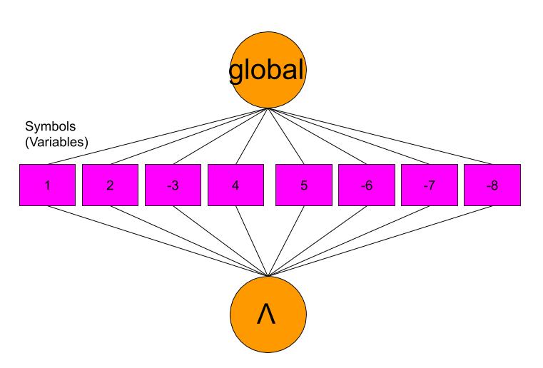
corresponding to one AND node and literals ‘i’ or ‘-i’:

where each clause is composed of only one variable.

It is then possible to use the graph embedder to compute an embedding representation for all assignments and compare them with the formula.

Satisfying assignment search

Positive assignments (propositions that make the formula True) are easier to search from the CNF format with the Solver from the PySat package. Clauses of CNF format are quite simple to express:

• in the case of the VRD dataset, each clause can be expressed in the code with a couple [-rel_id, pos_id] where rel_id is the ID of a relation predicate variable [relation predicate, subject, object] and pos_id is the ID of a spatial property variable [position relation, subject, object]. Variable ID are provided by variable ID manager pysat.formula.IDPool, always starting from 1.

• in the case of the synthetic dataset, a get_clauses() method parses the CNF clause list to return a list to map index to symbols (atom_mapping, for example ['e', 'f'] for a formula with e and f symbols) and a list of clauses in the format of lists as well: [-i] for a Not node, [i] for a symbol, and [(-)i, (-)j, (-)k, …] of an OR node where i, j, k are symbol indexes and (-) the Not operator.

5 positive assignments (propositions that make the formula True) are found with the Solver from the PySat package when the formula is of type pysat.formula.CNF. 5 negative assignments are easier to find by random tests.

During training, embedding of positive assignments are pushed to be closer to embedding of the formula than negative assignments are, thanks to a margin triplet loss based on the euclidian distance:

Features X of the formula graph nodes

The shape of input features X is (N, 50).

In the case of the synthetic dataset, node features come from model/pygcn/pygcn/features.pk file containing

• a list digit_to_sym to map index to symbol [None, 'a', 'b', 'c', 'd', 'e', 'f', 'g', 'h', 'i', 'j', 'k', 'l'] (None to have all symbol indexes greater or equal to 1)

• a type_map dictionary to map type to index: {'Global': 0, 'Symbol': 1, 'Or': 2, 'And': 3, 'Not': 4}

• a features dictionary containing a feature for each type and symbol Global, Symbol, Or, And, Not, a, b, c, d, e, f, g, h, i, j, k, l. Each feature is a numpy array of dimension (50,).

These features are randomly vectors, and the exchangeability of the variables ‘a, b, c, d, e, f, g, h, i, j, k, l’ will produce a network operating well on that manifold.

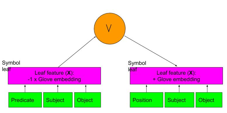
In the case of the VRD datasets,

• for nodes AND, OR, Global, features are reused from synthetic dataset.

• for Symbol leaf nodes which represent relation variables (relation, subject, object), GloVe vectors are used since they are semantic representations and may generalize to unseen propositions. Features are taken as the average of 50-dimensional Glove vectors for all words in the relation (predicate or position), subject and object names.

Most of objects and relations consisted of a single word. Potentially, the model could be improved via normalization, but it was experimented with that setting.

Training the logical embedder

An object MyDataset is implemented for the interface of torch.utils.data.DataLoader to deliver batches.

Each batch is composed of 5 items, where each item is a triplet of 3 elements (A, P, N): the anchor (the formula), the positive (or satisfying) assignment, a negative assignment. The three elements are used in the triplet margin loss: the positive assignment has to be closer to the formula than the negative assignment in the embedding space.

Each element are loaded from file with load_data function. It loads:

• node features (each line contains the id, features, label for each node)

• edges, converted into an adjacency matrix A, normalized with

The original ID are remapped to 0…N in the order the features are saved.

The return of the function composed of :

• adj: the NxN adjacency matrix in torch sparse float tensor,
• features: a dense float tensor with the features NxD,
• labels: a Nx1 dense long tensor,
• idx_train, idx_val, idx_test: NOT USED (simple range(0,N)),
• and_children, or_children: JSON load from file

The embedding is trained with triplet margin loss with euclidian distance, plus a semantic regularization loss that takes the 100-dimension embedding \(q_i\) of each children nodes of a AND or OR node and applies:

Q7: In the paper, the formula differs from code \(\displaystyle \sum_{\text{OR}} \| \sum_{j \in \text{children}} q(v_j) -1 \|_2^2 + \sum_{\text{AND}} \| V_k^T V_k - diag(V_k^T V_k) \|_2^2\)

The regularization loss is consistent with d-DNNF properties for AND and OR nodes, and is applied for d-DNNF only. Also, the paper shows it performs better when combined with heterogeneous node weights (different weights for AND and OR nodes).

Satifying assignments

A second network, a 2-layer MLP, is trained on top of embeddings \((E_f, E_P, E_N)\) to discriminate the satisfying assignment \((E_f, E_P)\) from the negative \((E_f, E_N)\) for the formula f.

Relation prediction

For the VRD experiment, a third network, a two-layer MLP, is trained to predict the relation.

The input of the MLP consists of the image features concatenated with Glove vectors for subject/object labels and relative position coordinates in the image crop. The output is a logit of dimension 71.

Input

For each subject-object pair, a feature vector is created by concatenating

• the image feature: a crop of the union of both bounding boxes is resized to 224x224, normalized, processed by the CV network to produce visual features from before last layer of ResNet 18 of dimension 512.

• word embeddings for both subject and object labels. word_embed.json contains GloVe word embeddings (dimension 300) for all object names.

• relative position coordinates of subject and object in the crop union of both bounding boxes.

The annotation key is given by

str((subject_category, subject_boundingbox),(object_category, object_boundingbox))

The concepts of subject and object are exchangeable, and a “no-relation-predicate” label is added to all void relations.

Each batch deals with one image only and the batch size is equal to the number of relations, negative relations subsampled.

Training loss

First, a Softmax+Crossentropy loss trains the network to predict the relation.

Second, thanks to a trained logical embedder that produces close embeddings for the formula and positive assignments, a logical loss can be applied to constrain the softmax of the logits to be close to the formula’s embeddings as well.

Since the softmax of the logits is not a boolean but a vector of probabilities for the 71 predicate variables, the feature of the symbol nodes in the assignment graph is replaced by an average of the word embeddings for predicate names weighted by the probabilities.

Optimizer applies gradients on the MLP model only, constraining only the MLP weights for the ouput to follow the embedder loss.

Well done!