UPDATE! : my Fast Image Annotation Tool for Caffe has just been released ! Have a look !

Caffe is certainly one of the best frameworks for deep learning, if not the best.

Let’s try to put things into order, in order to get a good tutorial :).

Caffe

Install

First install Caffe following my tutorials on Ubuntu or Mac OS with Python layers activated and pycaffe path correctly set export PYTHONPATH=~/technologies/caffe/python/:$PYTHONPATH.

Launch the python shell

In the iPython shell in your Caffe repository, load the different libraries :

import numpy as np
import matplotlib.pyplot as plt
from PIL import Image
import caffe

Set the computation mode CPU

caffe.set_mode_cpu()

or GPU

caffe.set_device(0)
caffe.set_mode_gpu()

Define a network model

Let’s create first a very simple model with a single convolution composed of 3 convolutional neurons, with kernel of size 5x5 and stride of 1 :

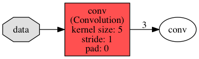
This net will produce 3 output maps from an input map.

The output map for a convolution given receptive field size has a dimension given by the following equation :

output = (input - kernel_size) / stride + 1

Create a first file conv.prototxt describing the neuron network :

name: "convolution"
input: "data"
input_dim: 1
input_dim: 1
input_dim: 100
input_dim: 100
layer {
  name: "conv"
  type: "Convolution"
  bottom: "data"
  top: "conv"
  convolution_param {
    num_output: 3
    kernel_size: 5
    stride: 1
    weight_filler {
      type: "gaussian"
      std: 0.01
    }
    bias_filler {
      type: "constant"
      value: 0
    }
  }
}

with one layer, a convolution, from the Catalog of available layers

Load the net

net = caffe.Net('conv.prototxt', caffe.TEST)

The names of input layers of the net are given by print net.inputs.

The net contains two ordered dictionaries

• net.blobs for input data and its propagation in the layers :

  net.blobs['data'] contains input data, an array of shape (1, 1, 100, 100) net.blobs['conv'] contains computed data in layer ‘conv’ (1, 3, 96, 96)

  initialiazed with zeros.

  To print the infos,

    [(k, v.data.shape) for k, v in net.blobs.items()]
  

• net.params a vector of blobs for weight and bias parameters

  net.params['conv'][0] contains the weight parameters, an array of shape (3, 1, 5, 5) net.params['conv'][1] contains the bias parameters, an array of shape (3,)

  initialiazed with ‘weight_filler’ and ‘bias_filler’ algorithms.

  To print the infos :

    [(k, v[0].data.shape, v[1].data.shape) for k, v in net.params.items()]
  

Blobs are memory abstraction objects (with execution depending on the mode), and data is contained in the field data as an array :

print net.blobs['conv'].data.shape

To draw the network, a simle python command :

python python/draw_net.py examples/net_surgery/conv.prototxt my_net.png
open my_net.png

This will print the following image :

Compute the net output on an image as input

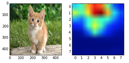
Let’s load a gray image of size 1x360x480 (channel x height x width) into the previous net :

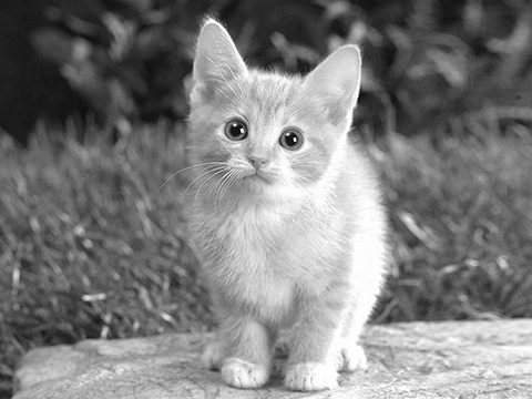
We need to reshape the data blob (1, 1, 100, 100) to the new size (1, 1, 360, 480) to fit the image :

im = np.array(Image.open('examples/images/cat_gray.jpg'))
im_input = im[np.newaxis, np.newaxis, :, :]
net.blobs['data'].reshape(*im_input.shape)
net.blobs['data'].data[...] = im_input

Let’s compute the blobs given this input

net.forward()

Now net.blobs['conv'] is filled with data, and the 3 pictures inside each of the 3 neurons (net.blobs['conv'].data[0,i]) can be plotted easily.

To save the net parameters net.params, just call :

net.save('mymodel.caffemodel')

Load pretrained parameters to classify an image

In the previous net, weight and bias params have been initialiazed randomly.

It is possible to load trained parameters and in this case, the result of the net will produce a classification.

Many trained models can be downloaded from the community in the Caffe Model Zoo, such as car classification, flower classification, digit classification…

Model informations are written in Github Gist format. The parameters are saved in a .caffemodel file specified in the gist. To download the model :

./scripts/download_model_from_gist.sh <gist_id>
./scripts/download_model_binary.py <dirname>

where is the gist directory (by default the gist is saved in the *models* directory).

Let’s download the CaffeNet model and the labels corresponding to the classes :

./scripts/download_model_binary.py models/bvlc_reference_caffenet
./data/ilsvrc12/get_ilsvrc_aux.sh

#have a look at the model
python python/draw_net.py models/bvlc_reference_caffenet/deploy.prototxt caffenet.png
open caffenet.png

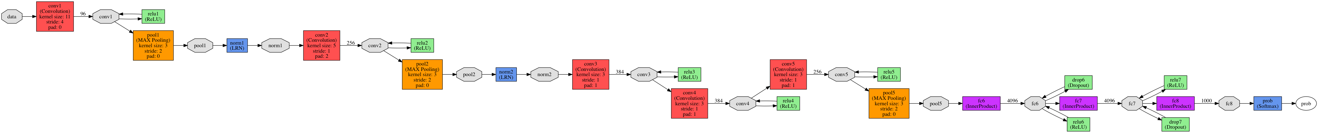
This model has been trained on processed images, so you need to preprocess the image with a preprocessor, before saving it in the blob.

That is, in the python shell :

#load the model
net = caffe.Net('models/bvlc_reference_caffenet/deploy.prototxt',
                'models/bvlc_reference_caffenet/bvlc_reference_caffenet.caffemodel',
                caffe.TEST)

# load input and configure preprocessing
transformer = caffe.io.Transformer({'data': net.blobs['data'].data.shape})
transformer.set_mean('data', np.load('python/caffe/imagenet/ilsvrc_2012_mean.npy').mean(1).mean(1))
transformer.set_transpose('data', (2,0,1))
transformer.set_channel_swap('data', (2,1,0))
transformer.set_raw_scale('data', 255.0)

#note we can change the batch size on-the-fly
#since we classify only one image, we change batch size from 10 to 1
net.blobs['data'].reshape(1,3,227,227)

#load the image in the data layer
im = caffe.io.load_image('examples/images/cat.jpg')
net.blobs['data'].data[...] = transformer.preprocess('data', im)

#compute
out = net.forward()

# other possibility : out = net.forward_all(data=np.asarray([transformer.preprocess('data', im)]))

#predicted predicted class
print out['prob'].argmax()

#print predicted labels
labels = np.loadtxt("data/ilsvrc12/synset_words.txt", str, delimiter='\t')
top_k = net.blobs['prob'].data[0].flatten().argsort()[-1:-6:-1]
print labels[top_k]

It will print you the top classes detected for the images.

Go further : Create a classification map with net surgery to insert a trained model into an extended model where convolutions will be innerproducts spatially

Learn : solve the params on training data

It is now time to create your own model, and training the parameters on training data.

To train a network, you need

• its model definition, as seen previously

• a second protobuf file, the solver file, describing the parameters for the stochastic gradient.

For example, the CaffeNet solver :

net: "models/bvlc_reference_caffenet/train_val.prototxt"
test_iter: 1000
test_interval: 1000
base_lr: 0.01
lr_policy: "step"
gamma: 0.1
stepsize: 100000
display: 20
max_iter: 450000
momentum: 0.9
weight_decay: 0.0005
snapshot: 10000
snapshot_prefix: "models/bvlc_reference_caffenet/caffenet_train"
solver_mode: GPU

Usually, you define a train net, for training, with training data, and a test set, for validation. Either you can define the train and test nets in the prototxt solver file

train_net: "examples/hdf5_classification/nonlinear_auto_train.prototxt"
test_net: "examples/hdf5_classification/nonlinear_auto_test.prototxt"

or you can also specify only one prototxt file, adding an include phase statement for the layers that have to be different in training and testing phases, such as input data :

layer {
  name: "data"
  type: "Data"
  top: "data"
  top: "label"
  include {
    phase: TRAIN
  }
  data_param {
    source: "examples/imagenet/ilsvrc12_train_lmdb"
    batch_size: 256
    backend: LMDB
  }
}
layer {
  name: "data"
  type: "Data"
  top: "data"
  top: "label"
  top: "label"
  include {
    phase: TEST
  }
  data_param {
    source: "examples/imagenet/ilsvrc12_val_lmdb"
    batch_size: 50
    backend: LMDB
  }
}

Data can also be set directly in Python.

Load the solver in python

solver = caffe.get_solver('models/bvlc_reference_caffenet/solver.prototxt')

By default it is the SGD solver. It’s possible to specify another solver_type in the prototxt solver file (ADAGRAD or NESTEROV). It’s also possible to load directly

solver = caffe.SGDSolver('models/bvlc_reference_caffenet/solver.prototxt')

but be careful since SGDSolver will use SGDSolver whatever is configured in the prototxt file… so it is less reliable.

Now, it’s time to begin to see if everything works well and to fill the layers in a forward propagation in the net (computation of net.blobs[k].data from input layer until the loss layer) :

solver.net.forward()  # train net
solver.test_nets[0].forward()  # test net (there can be more than one)

For the computation of the gradients (computation of the net.blobs[k].diff and net.params[k][j].diff from the loss layer until input layer) :

solver.net.backward()

To launch one step of the gradient descent, that is a forward propagation, a backward propagation and the update of the net params given the gradients (update of the net.params[k][j].data) :

solver.step(1)

To run the full gradient descent, that is the max_iter steps :

solver.solve()

Input data, train and test set

In order to learn a model, you usually set a training set and a test set.

The different input layer can be :

• ‘Data’ : for data saved in a LMDB database, such as before

• ‘ImageData’ : for data in a txt file listing all the files

    layer {
      name: "data"
      type: "ImageData"
      top: "data"
      top: "label"
      transform_param {
        mirror: false
        crop_size: 227
        mean_file: "data/ilsvrc12/imagenet_mean.binaryproto"
      }
      image_data_param {
        source: "examples/_temp/file_list.txt"
        batch_size: 50
        new_height: 256
        new_width: 256
      }
    }
  

• ‘HDF5Data’ for data saved in HDF5 files

    layer {
      name: "data"
      type: "HDF5Data"
      top: "data"
      top: "label"
      hdf5_data_param {
        source: "examples/hdf5_classification/data/train.txt"
        batch_size: 10
      }
    }
  

Compute accuracy of the model on the test data

Once solved,

accuracy = 0
batch_size = solver.test_nets[0].blobs['data'].num
test_iters = int(len(Xt) / batch_size)
for i in range(test_iters):
    solver.test_nets[0].forward()
    accuracy += solver.test_nets[0].blobs['accuracy'].data
accuracy /= test_iters

print("Accuracy: {:.3f}".format(accuracy))

The higher the accuracy, the better !

Parameter sharing

Parameter sharing between Siamese networks

Recurrent neural nets in Caffe

Have a look at my tutorial about recurrent neural nets in Caffe.

Spatial transformer layers

my tutorial about improving classification with spatial transformer layers

Caffe in Python

Define a model in Python

It is also possible to define the net model directly in Python, and save it to a prototxt files. Here are the commands :

from caffe import layers as L
from caffe import params as P

def lenet(lmdb, batch_size):
    # our version of LeNet: a series of linear and simple nonlinear transformations
    n = caffe.NetSpec()
    n.data, n.label = L.Data(batch_size=batch_size, backend=P.Data.LMDB, source=lmdb,
                             transform_param=dict(scale=1./255), ntop=2)
    n.conv1 = L.Convolution(n.data, kernel_size=5, num_output=20, weight_filler=dict(type='xavier'))
    n.pool1 = L.Pooling(n.conv1, kernel_size=2, stride=2, pool=P.Pooling.MAX)
    n.conv2 = L.Convolution(n.pool1, kernel_size=5, num_output=50, weight_filler=dict(type='xavier'))
    n.pool2 = L.Pooling(n.conv2, kernel_size=2, stride=2, pool=P.Pooling.MAX)
    n.ip1 = L.InnerProduct(n.pool2, num_output=500, weight_filler=dict(type='xavier'))
    n.relu1 = L.ReLU(n.ip1, in_place=True)
    n.ip2 = L.InnerProduct(n.relu1, num_output=10, weight_filler=dict(type='xavier'))
    n.loss = L.SoftmaxWithLoss(n.ip2, n.label)
    return n.to_proto()

with open('examples/mnist/lenet_auto_train.prototxt', 'w') as f:
    f.write(str(lenet('examples/mnist/mnist_train_lmdb', 64)))

with open('examples/mnist/lenet_auto_test.prototxt', 'w') as f:
    f.write(str(lenet('examples/mnist/mnist_test_lmdb', 100)))

will produce the prototxt file :

layer {
  name: "data"
  type: "Data"
  top: "data"
  top: "label"
  transform_param {
    scale: 0.00392156862745
  }
  data_param {
    source: "examples/mnist/mnist_train_lmdb"
    batch_size: 64
    backend: LMDB
  }
}
layer {
  name: "conv1"
  type: "Convolution"
  bottom: "data"
  top: "conv1"
  convolution_param {
    num_output: 20
    kernel_size: 5
    weight_filler {
      type: "xavier"
    }
  }
}
layer {
  name: "pool1"
  type: "Pooling"
  bottom: "conv1"
  top: "pool1"
  pooling_param {
    pool: MAX
    kernel_size: 2
    stride: 2
  }
}
layer {
  name: "conv2"
  type: "Convolution"
  bottom: "pool1"
  top: "conv2"
  convolution_param {
    num_output: 50
    kernel_size: 5
    weight_filler {
      type: "xavier"
    }
  }
}
layer {
  name: "pool2"
  type: "Pooling"
  bottom: "conv2"
  top: "pool2"
  pooling_param {
    pool: MAX
    kernel_size: 2
    stride: 2
  }
}
layer {
  name: "ip1"
  type: "InnerProduct"
  bottom: "pool2"
  top: "ip1"
  inner_product_param {
    num_output: 500
    weight_filler {
      type: "xavier"
    }
  }
}
layer {
  name: "relu1"
  type: "ReLU"
  bottom: "ip1"
  top: "ip1"
}
layer {
  name: "ip2"
  type: "InnerProduct"
  bottom: "ip1"
  top: "ip2"
  inner_product_param {
    num_output: 10
    weight_filler {
      type: "xavier"
    }
  }
}
layer {
  name: "loss"
  type: "SoftmaxWithLoss"
  bottom: "ip2"
  bottom: "label"
  top: "loss"
}

Create your custom python layer

Let’s create a layer to add a value.

Add a custom python layer to your conv.prototxt file :

layer {
  name: 'MyPythonLayer'
  type: 'Python'
  top: 'output'
  bottom: 'conv'
  python_param {
    module: 'mypythonlayer'
    layer: 'MyLayer'
    param_str: "'num': 21"
  }
}

and create a mypythonlayer.py file that has to to be in the current directory or in the PYTHONPATH :

import caffe
import numpy as np
import yaml

class MyLayer(caffe.Layer):

    def setup(self, bottom, top):
        self.num = yaml.load(self.param_str)["num"]
        print "Parameter num : ", self.num

    def reshape(self, bottom, top):
        pass

    def forward(self, bottom, top):
        top[0].reshape(*bottom[0].shape)
        top[0].data[...] = bottom[0].data + self.num

    def backward(self, top, propagate_down, bottom):
        pass

This layer will simply add a value

net = caffe.Net('conv.prototxt',caffe.TEST)
im = np.array(Image.open('cat_gray.jpg'))
im_input = im[np.newaxis, np.newaxis, :, :]
net.blobs['data'].reshape(*im_input.shape)
net.blobs['data'].data[...] = im_input
net.forward()

Caffe in C++

The blob

The blob (blob.hpp and blob.cpp) is a wrapper to manage memory independently of CPU/GPU choice, using SyncedMemory class, and has a few functions like Arrays in Python, both for the data and the computed gradient (diff) arrays contained in the blob.

To initiate a blob :

Blob(const vector<int>& shape)

Methods on the blob :

• shape() and shape_string() to get the shape, or shape(i) to get the size of the i-th dimension, or shapeEquals() to compare shape equality
• Reshape(const vector<int>& shape) or reshapeLike(const Blob& other) another blob
• count() the number of elements (shape(0)*shape(1)*...)
• offset() to get the c++ index in the array
• CopyFrom() to copy the blob
• data_at() and diff_at()
• asum_data() and asum_diff() their L1 norm
• sumsq_data() and sumsq_diff() their L1 norm
• scale_data() and scale_diff() to multiply the data by a factor
• Update() to update data array given diff array

To access the data in the blob, from the CPU code :

const Dtype* cpu_data();
Dtype* mutable_cpu_data();
const Dtype* cpu_diff();
Dtype* mutable_cpu_diff();

and from the GPU code :

const Dtype* gpu_data();
Dtype* mutable_gpu_data();
const Dtype* gpu_diff();
Dtype* mutable_gpu_diff();

Data transfer between GPU and CPU will be dealt automatically.

Caffe provides abstraction methods to deal with data :

• caffe_set() and caffe_gpu_set() to initialize the data with a value

• caffe_add_scalar() and caffe_gpu_add_scalar() to add a scalar to data

• caffe_axpy() and caffe_gpu_axpy() for \(y \leftarrow a x + y\)

• caffe_scal() and caffe_gpu_scal() for \(x \leftarrow a x\)

• caffe_cpu_sign() and caffe_gpu_sign() for \(y \leftarrow \text{sign} (x)\)

• caffe_cpu_axpby() and caffe_cpu_axpby for \(y \leftarrow a \times x + b \times y\)

• caffe_copy() to deep copy

• caffe_cpu_gemm() and caffe_gpu_gemm() for matrix multiplication \(C \leftarrow \alpha A \times B + \beta C\)

• caffe_gpu_atomic_add() when you need to update a value in an atomic way (such as requests in ACID databases but for gpu threads in this case)

… and so on.

The layer

A layer, such as the SoftmaxWithLoss layer, will need a few functions working with arguments top blobs and bottom blobs :

• Forward_cpu or Forward_gpu
• Backward_cpu or Backward_gpu
• Reshape
• optionaly : LayerSetUp, to set non-standard fields

The layer_factory is a set of helper functions to get the right layer implementation according to the engine (Caffe or CUDNN).