It is not straightforward to understand the torch.rnn package since it begins the description with abstract classes.

Let’s begin with simple examples and put things back into order to simplify comprehension for beginners.

In this tutorial, I will also translate the Keras LTSM or Theano LSTM examples to Torch.

Install

To use Torch with NVIDIA library CUDA, I would advise to copy the CUDA files to a new directory /usr/local/cuda-8-cudnn-5 in which you install the last CUDNN since Torch prefers a CUDNN version above 5. The install guide will step up Torch. In your ~/.bashrc :

export LD_LIBRARY_PATH=/usr/local/cuda-8.0-cudnn-5/lib64:/usr/local/cuda-8.0-cudnn-4/lib64:/usr/local/lib/
. /home/christopher/torch/install/bin/torch-activate

Install the rnn package and the dependencies

luarocks install torch
luarocks install nn
luarocks install dpnn
luarocks install torchx
luarocks install cutorch
luarocks install cunn
luarocks install cunnx
luarocks install rnn

Launch a Torch shell with luajit command.

Build a simple RNN

Let’s build a simple RNN like this one :

simple RNN

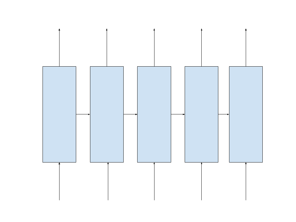
with an hidden state of size 7 to predict the new word in a dictionary of 10 words.

In this example, the RNN remembers the last 5 steps or words in our sequence. So, the backpropagation through time will be limited to the last 5 steps.

1. Compute the hidden state at each time step

A recurrent net is a net that take its previous internal state and optionally an input to compute its new state :

\[h_t = \sigma(W_{hh} h_{t−1} + W_{xh} X_t)\]

The \(W_{xh}\) is a kind of word embedding where the multiplication with the word one-hot encoding selects the vector representing the word in the embedding space (in this case it’s a 7-dim space). Thanks to nn.LookupTable, you don’t need to convert your words into one-hot encoding, you just provide the word index as input.

In Torch RNN, this equation is implemened by the nn.Reccurent layer which output is the state :

require 'rnn'

r = nn.Recurrent(
    7,
    nn.LookupTable(10, 7),
    nn.Linear(7, 7),
    nn.Sigmoid(),
    5
  )
=r

The nn.Recurrent takes 6 arguments :

7, the size of the hidden state
nn.LookupTable(10, 7) computing the impact of the input \(W_{xh} X_t\)
nn.Linear(7, 7) describing the impact of the previous state \(W_{hh} h_{t−1}\)
nn.Sigmoid() the non-linearity or activation function, also named transfer function
5 (the rho parameter) is the maximum number of steps to backpropagate through time (BPPT). It can be initialiazed to 9999 or the size of the sequence.

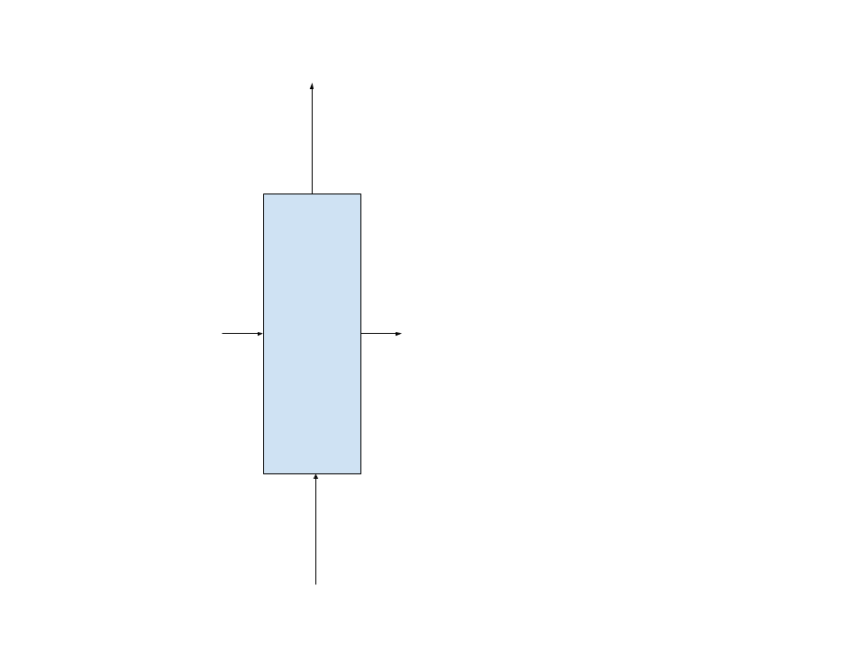
So far, we have built this part of our target RNN :

simple RNN

This module inherits from the AbstractRecurrent interface (abstract class).

There is an alternative way to create the same net, thanks to a more general module, nn.Recurrence :

rm = nn.Sequential()
   :add(nn.ParallelTable()
      :add(nn.LookupTable(10, 7))
      :add(nn.Linear(7, 7)))
   :add(nn.CAddTable())
   :add(nn.Sigmoid())

r = nn.Recurrence(rm, 7, 1)   

where

rm has to be a module that computes \(h_t\) given an input table \(X_t, h_{t-1}\)
7 is the hidden state size
1 is the input dimension

2. Compute the output at a time step

Now, let’s add the output to our previous net.

Output is computed thanks to

\[o_t = W_{ho} h_t\]

and converted to a probability with the log softmax function.

rr = nn.Sequential()
   :add(r)
   :add(nn.Linear(7, 10))
   :add(nn.LogSoftMax())
=rr

Now, our module will look like this, that is a complete step :

simple RNN

This module does not inherit anymore from the AbstractRecurrent interface (abstract class).

3. Make it a recurrent module / RNN

The previous module is not recurrent. It can still take one input at time, but without the convenient methods to train it through time.

Recurrent, LSTM, GRU, … are recurrent modules but Linear and LogSoftMax are not.

Since we added non-recurrent modules, we have to transform the net back to a recurrent module, with the Recursor function :

rnn = nn.Recursor(rr, 5)
=rnn

This will clone the non-recurrent submodules for the number of steps the net has to remember for retropropagation through time (BPTT), each clone sharing the same parameters and gradients for the parameters.

Now we have a net with the capacity to remember the last 5 steps for training :

simple RNN

This module inherits from the AbstractRecurrent interface (abstract class).

4. Apply each element of a sequence to the RNN step by step

Let’s apply our recurring net to a sequence of 5 words given by an input torch.LongTensor and compute the error with the expected target torch.LongTensor.

outputs, err = {}, 0
criterion = nn.ClassNLLCriterion()
for step=1,5 do
   outputs[step] = rnn:forward(inputs[step])
   err = err + criterion:forward(outputs[step], targets[step])
end

5. Train the RNN step by step through the sequence

Let’s retropropagate the error through time, going in the reverse order of the forwards:

gradOutputs, gradInputs = {}, {}
for step=5,1,-1 do
  gradOutputs[step] = criterion:backward(outputs[step], targets[step])
  gradInputs[step] = rnn:backward(inputs[step], gradOutputs[step])
end

and update the parameters

rnn:updateParameters(0.1) -- learning rate

6. Reset the RNN

To reset the hidden state once training or evaluation of a sequence is done :

rnn:forget()

to forward a new sequence.

To reset the accumulated gradients for the parameters once training of a sequence is done :

rnn:zeroGradParameters()

for backpropagation through a new sequence.

Apply RNN to a sequence in one step thanks to sequencer module

The Sequencer module enables to transform a net to apply it directly to the full sequence:

rnn = nn.Sequencer(rr)
criterion = nn.SequencerCriterion(nn.ClassNLLCriterion())

which is the same as rnn = nn.Sequencer(nn.Recursor(rr)) because the sequence does it internally.

Then, there is only one global forward and backward pass as if it were a feedforward net :

outputs = rnn:forward(inputs)
err = criterion:forward(outputs, targets)
gradOutputs = criterion:backward(outputs, targets)
gradInputs = rnn:backward(inputs, gradOutputs)
rnn:updateParameters(0.1)

Since the Sequencer takes care of calling the forget method, just reset the gradient parameters for the next training step :

rnn:zeroGradParameters()

Regularize RNN

To regularize the hidden states of the RNN by adding a norm-stabilization criterion, add :

rr:add(nn.NormStabilizer())

Prebuilt RNN and Sequencers

There exists a bunch of prebuilt RNN :

nn.LSTM and nn.FastLSTM (a faster version)
nn.GRU

as well as sequencers :

nn.seqLSTM (a faster version than nn.Sequencer(nn.FastLSTM))
nn.seqGRU
nn.BiSequencer to transform a RNN into a bidirectionnal RNN
nn.SeqBRNN a bidirectionnal LSTM
nn.Repeater a simple repeat layer (which is not a RNN)
nn.RecurrentAttention

Helper functions

nn.SeqReverseSequence to reverse a sequence order
n.SequencerCriterion
nn.RepeaterCriterion

Full documentation is available here.

Example

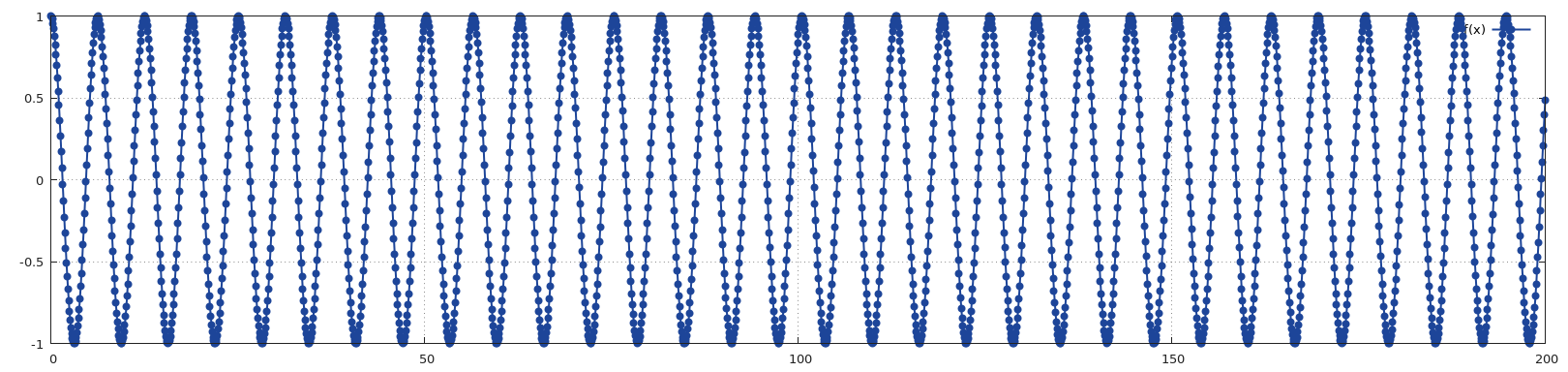
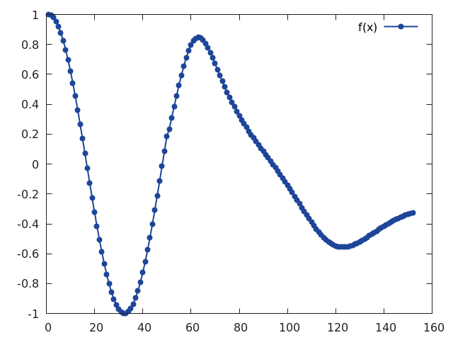
Let’s try to predict a cos function with our RNN :

require 'torch'
require 'gnuplot'
ii=torch.linspace(0,200, 2000)
oo=torch.cos(ii)
gnuplot.plot({'f(x)',ii,oo,'+-'})

In this case, I’m only interested in predicting the value at the last step, and do not need to use a sequencer for the criterion :

require 'rnn'
require 'gnuplot'

gpu=1
if gpu>0 then
  print("CUDA ON")
  require 'cutorch'
  require 'cunn'
  cutorch.setDevice(gpu)
end

nIters = 2000
batchSize = 80
rho = 10
hiddenSize = 300
nIndex = 1
lr = 0.0001
nPredict=200

rnn = nn.Sequential()
   :add(nn.Linear(nIndex, hiddenSize))
   :add(nn.FastLSTM(hiddenSize, hiddenSize))
   :add(nn.NormStabilizer())
   :add(nn.Linear(hiddenSize, nIndex))
   :add(nn.HardTanh())
rnn = nn.Sequencer(rnn)
rnn:training()
print(rnn)

if gpu>0 then
  rnn=rnn:cuda()
end

criterion = nn.MSECriterion()
if gpu>0 then
  criterion=criterion:cuda()
end

ii=torch.linspace(0,200, 2000)
sequence=torch.cos(ii)
if gpu>0 then
  sequence=sequence:cuda()
end

offsets = {}
for i=1,batchSize do
   table.insert(offsets, math.ceil(math.random()* (sequence:size(1)-rho) ))
end
offsets = torch.LongTensor(offsets)
if gpu>0 then
  offsets=offsets:cuda()
end

local gradOutputsZeroed = {}
for step=1,rho do
  gradOutputsZeroed[step] = torch.zeros(batchSize,1)
  if gpu>0 then
    gradOutputsZeroed[step] = gradOutputsZeroed[step]:cuda()
  end
end

local iteration = 1
while iteration < nIters do
   local inputs, targets = {}, {}
   for step=1,rho do
      inputs[step] = sequence:index(1, offsets):view(batchSize,1)
      offsets:add(1)
      for j=1,batchSize do
         if offsets[j] > sequence:size(1) then
            offsets[j] = 1
         end
      end
      targets[step] = sequence:index(1, offsets)
   end
   rnn:zeroGradParameters()
   local outputs = rnn:forward(inputs)
   local err = criterion:forward(outputs[rho], targets[rho])
   print(string.format("Iteration %d ; NLL err = %f ", iteration, err))
   local gradOutputs = criterion:backward(outputs[rho], targets[rho])
   gradOutputsZeroed[rho] = gradOutputs
   local gradInputs = rnn:backward(inputs, gradOutputsZeroed)
   rnn:updateParameters(lr)
   iteration = iteration + 1
end

rnn:evaluate()
predict=torch.FloatTensor(nPredict)
if gpu>0 then
  predict=predict:cuda()
end
for step=1,rho do
  predict[step]= sequence[step]
end

start = {}
iteration=0
while rho + iteration < nPredict do
  for step=1,rho do
    start[step] = predict:index(1,torch.LongTensor({step+iteration})):view(1,1)
  end

  output = rnn:forward(start)

  predict[iteration+rho+1] = (output[rho]:float())[1][1]

  iteration = iteration + 1
end

gnuplot.plot({'f(x)',predict,'+-'})

I get a very nice gradient descent :

nn.Sequencer @ nn.Recursor @ nn.Sequential {
  [input -> (1) -> (2) -> (3) -> (4) -> output]
  (1): nn.Linear(1 -> 300)
  (2): nn.FastLSTM(300 -> 300)
  (3): nn.Linear(300 -> 1)
  (4): nn.HardTanh
}
Iteration 1 ; NLL err = 3.478229
Iteration 2 ; NLL err = 4.711619
Iteration 3 ; NLL err = 4.542660
Iteration 4 ; NLL err = 3.371824
Iteration 5 ; NLL err = 4.201443
Iteration 6 ; NLL err = 4.436131
Iteration 7 ; NLL err = 3.094949
Iteration 8 ; NLL err = 3.780032
Iteration 9 ; NLL err = 4.248514
Iteration 10 ; NLL err = 3.110518
Iteration 11 ; NLL err = 3.369119
Iteration 12 ; NLL err = 4.055705
Iteration 13 ; NLL err = 2.945628
Iteration 14 ; NLL err = 2.976552
Iteration 15 ; NLL err = 3.823381
Iteration 16 ; NLL err = 2.986773
Iteration 17 ; NLL err = 2.727758
Iteration 18 ; NLL err = 3.539114
Iteration 19 ; NLL err = 2.894664
Iteration 20 ; NLL err = 2.383644
Iteration 21 ; NLL err = 3.300501
Iteration 22 ; NLL err = 2.888519
Iteration 23 ; NLL err = 2.401882
Iteration 24 ; NLL err = 2.519863
Iteration 25 ; NLL err = 2.994562
Iteration 26 ; NLL err = 2.299234
Iteration 27 ; NLL err = 2.321184
Iteration 28 ; NLL err = 2.882515
Iteration 29 ; NLL err = 2.376524
Iteration 30 ; NLL err = 2.073522
Iteration 31 ; NLL err = 2.610386
Iteration 32 ; NLL err = 2.295232
Iteration 33 ; NLL err = 1.823012
Iteration 34 ; NLL err = 2.172308
Iteration 35 ; NLL err = 2.719259
Iteration 36 ; NLL err = 1.604506
Iteration 37 ; NLL err = 1.713154
Iteration 38 ; NLL err = 2.718607
Iteration 39 ; NLL err = 1.622171
Iteration 40 ; NLL err = 1.564815
Iteration 41 ; NLL err = 2.595195
Iteration 42 ; NLL err = 1.911170
Iteration 43 ; NLL err = 1.026671
Iteration 44 ; NLL err = 2.212237
Iteration 45 ; NLL err = 2.044593
Iteration 46 ; NLL err = 1.048580
Iteration 47 ; NLL err = 2.042109
Iteration 48 ; NLL err = 2.183428
Iteration 49 ; NLL err = 0.942648
Iteration 50 ; NLL err = 1.632405
Iteration 51 ; NLL err = 2.064977
Iteration 52 ; NLL err = 1.030269
Iteration 53 ; NLL err = 1.481484
Iteration 54 ; NLL err = 2.120936
Iteration 55 ; NLL err = 1.045050
Iteration 56 ; NLL err = 1.143302
Iteration 57 ; NLL err = 1.915937
Iteration 58 ; NLL err = 1.136797
Iteration 59 ; NLL err = 1.057004
Iteration 60 ; NLL err = 1.887239
Iteration 61 ; NLL err = 1.220893
Iteration 62 ; NLL err = 0.813717
Iteration 63 ; NLL err = 1.633107
Iteration 64 ; NLL err = 1.265849
Iteration 65 ; NLL err = 0.807005
Iteration 66 ; NLL err = 1.549983
Iteration 67 ; NLL err = 1.363749
Iteration 68 ; NLL err = 0.663062
Iteration 69 ; NLL err = 1.287098
Iteration 70 ; NLL err = 1.337819
Iteration 71 ; NLL err = 0.813959
Iteration 72 ; NLL err = 1.087296
Iteration 73 ; NLL err = 1.330080
Iteration 74 ; NLL err = 0.812519
Iteration 75 ; NLL err = 0.887653
Iteration 76 ; NLL err = 1.243328
Iteration 77 ; NLL err = 0.876112
Iteration 78 ; NLL err = 0.864694
Iteration 79 ; NLL err = 1.211960
Iteration 80 ; NLL err = 0.856085
Iteration 81 ; NLL err = 0.717277
Iteration 82 ; NLL err = 1.075117
Iteration 83 ; NLL err = 0.915106
Iteration 84 ; NLL err = 0.720896
Iteration 85 ; NLL err = 1.039277
Iteration 86 ; NLL err = 0.906145
Iteration 87 ; NLL err = 0.622168
Iteration 88 ; NLL err = 0.884353
Iteration 89 ; NLL err = 0.935744
Iteration 90 ; NLL err = 0.650118
Iteration 91 ; NLL err = 0.857103
Iteration 92 ; NLL err = 0.922935
Iteration 93 ; NLL err = 0.590617
Iteration 94 ; NLL err = 0.714091
Iteration 95 ; NLL err = 0.906052
Iteration 96 ; NLL err = 0.636926
Iteration 97 ; NLL err = 0.702802
Iteration 98 ; NLL err = 0.885057
Iteration 99 ; NLL err = 0.604726
Iteration 100 ; NLL err = 0.588609
Iteration 101 ; NLL err = 0.821450
Iteration 102 ; NLL err = 0.658520
Iteration 103 ; NLL err = 0.594702
Iteration 104 ; NLL err = 0.798030
Iteration 105 ; NLL err = 0.640358
Iteration 106 ; NLL err = 0.512068
Iteration 107 ; NLL err = 0.703881
Iteration 108 ; NLL err = 0.684981
Iteration 109 ; NLL err = 0.604532
Iteration 110 ; NLL err = 0.636330
Iteration 111 ; NLL err = 0.639078
Iteration 112 ; NLL err = 0.547678
Iteration 113 ; NLL err = 0.547235
Iteration 114 ; NLL err = 0.678862
Iteration 115 ; NLL err = 0.560977
Iteration 116 ; NLL err = 0.569446
Iteration 117 ; NLL err = 0.619529
Iteration 118 ; NLL err = 0.523523
Iteration 119 ; NLL err = 0.499097
Iteration 120 ; NLL err = 0.618974
Iteration 121 ; NLL err = 0.552927
Iteration 122 ; NLL err = 0.524827
Iteration 123 ; NLL err = 0.580320
Iteration 124 ; NLL err = 0.509551
Iteration 125 ; NLL err = 0.542031
Iteration 126 ; NLL err = 0.505177
Iteration 127 ; NLL err = 0.526070
Iteration 128 ; NLL err = 0.550887
Iteration 129 ; NLL err = 0.506778
Iteration 130 ; NLL err = 0.496626
Iteration 131 ; NLL err = 0.496177
Iteration 132 ; NLL err = 0.459614
Iteration 133 ; NLL err = 0.512970
Iteration 134 ; NLL err = 0.510200
Iteration 135 ; NLL err = 0.493927
Iteration 136 ; NLL err = 0.478242
Iteration 137 ; NLL err = 0.469066
Iteration 138 ; NLL err = 0.438251
Iteration 139 ; NLL err = 0.491760
Iteration 140 ; NLL err = 0.470696
Iteration 141 ; NLL err = 0.488973
Iteration 142 ; NLL err = 0.458510
Iteration 143 ; NLL err = 0.444725
Iteration 144 ; NLL err = 0.434091
Iteration 145 ; NLL err = 0.456029
Iteration 146 ; NLL err = 0.507002
Iteration 147 ; NLL err = 0.471493
Iteration 148 ; NLL err = 0.405813
Iteration 149 ; NLL err = 0.461068
Iteration 150 ; NLL err = 0.426678
Iteration 151 ; NLL err = 0.409109
Iteration 152 ; NLL err = 0.450131
Iteration 153 ; NLL err = 0.471058
Iteration 154 ; NLL err = 0.396857
Iteration 155 ; NLL err = 0.427719
Iteration 156 ; NLL err = 0.438204
Iteration 157 ; NLL err = 0.376211
Iteration 158 ; NLL err = 0.435599
Iteration 159 ; NLL err = 0.453306
Iteration 160 ; NLL err = 0.407634
Iteration 161 ; NLL err = 0.394030
Iteration 162 ; NLL err = 0.436184
Iteration 163 ; NLL err = 0.368198
Iteration 164 ; NLL err = 0.417756
Iteration 165 ; NLL err = 0.425213
Iteration 166 ; NLL err = 0.425733
Iteration 167 ; NLL err = 0.368773
Iteration 168 ; NLL err = 0.419775

In this example, I’m also using the GPU of my notebook

laptop ROG

compared with a CPU descent on a MacBook Pro or iMac:

GPU makes the difference !

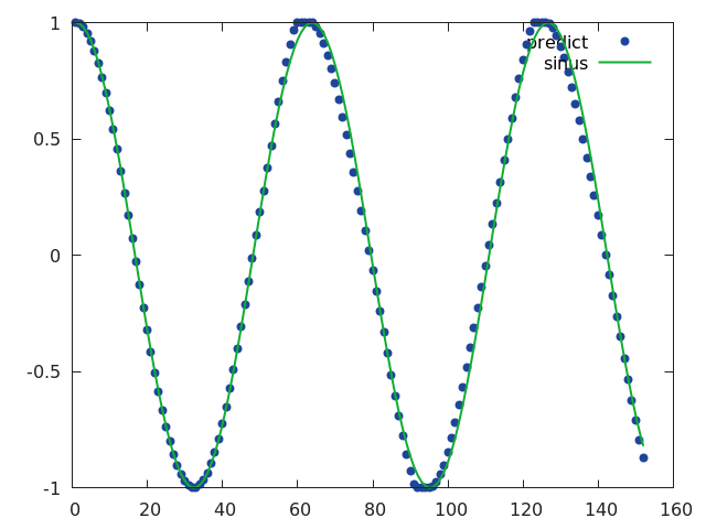
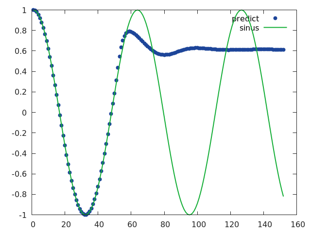
Eval one step

If you eval one step, then you get an impressive match, as many repositories do :

In this case, prediction is given based on a set of perfectly correct previous values.

Note that you can think of an algorithm that simply takes the last value of the input sequence as the prediction : this will produce a very good looking curve, with just a small delay. This means that predicting only one step is an easy task, and we won’t be able to judge the capacity of the network.

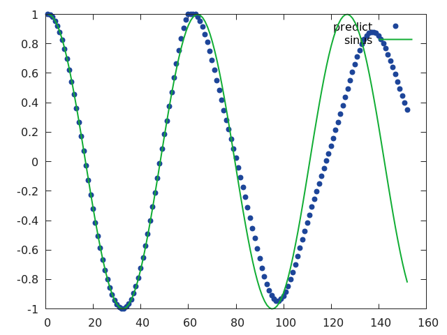
Eval multiple step ahead

I’d like to see how the prediction behaves when using the previous predicted values, and how error will be cumulated :

There is one limitation : training has not been done to consider this case of multiple step ahead previous predictions, even if dropout could help correct errors a bit. This gives a good reason to consider re-inforcement learning instead.

A few notes :

It is also possible to predict a value at each step and back propagate for all outputs. Except for the value 1 and -1, the network will never be able to predict correctly without history and reduce its error during the first steps.
It is absolutely not an optimal network for the problem. Just an example. Hyperparameter tuning will help find the correct coefficients.
We can see that even with errors in the past predictions, the network does not take any delay for the future.
It is always good to know where to put the gradients manually, but you can simplify the code by selecting only the last output with the nn.SelectTable module :

rnn = nn.FastLSTM(nIndex, hiddenSize)

rnn = nn.Sequential()
    :add(nn.SplitTable(0,2))
    :add(nn.Sequencer(rnn))
    :add(nn.SelectTable(-1))
    :add(nn.Linear(hiddenSize, hiddenSize))
    :add(nn.ReLU())
    :add(nn.Linear(hiddenSize, nIndex))
    :add(nn.Tanh())

Note also the use of nn.SplitTable to use a Tensor as input instead of a table.

Full code is available here.

option -select false to desactivate the use of nn.SelectTable in the model (does not change the computations).
option -eval_one_step true to evaluate only one step.

It is funny to play with the different parameters to see how it goes :

Well done!