In this article, I re-explain the characteristics of the bounding box object detector Yolo since everything might not be so easy to catch. Its first version has been improved in a version 2.

The network outputs’ grid

The convolutions enable to compute predictions at different positions in an image in an optimized way. This avoids using a sliding window to compute separately a prediction at every potential position.

The deep learning network for prediction is composed of convolution layers of stride 1, and max-pooling layers of stride 2 and kernel size 2.

To make it easier to align the grid of predictions produced by the network with the image:

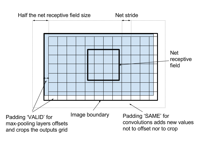
each max-pooling layer divides the output size by 2, multiplies the network stride by 2, and shifts the position in the image corresponding to the net receptive field center by 1 pixel. The padding mode used is ‘VALID’, meaning it is the floor division in the image size division, the extra values left on the right and the bottom of the image will only be used in the network field but a smaller image without these pixels (as the blue one in the figure below) would lead to the same grid;
the padding mode ‘SAME’ used in the convolutions means the output has the same size as the input. This is performed by padding with some zeros (or other new values) each border of the image. If we’d used a ‘VALID’ padding for the convolutions, then the first position on the grid would be shifted by half the network reception field size, which can be huge (~ 200 pixels for a ~400 pixel large network). The problem requires us to predict objects close to the borders, so, to avoid a shift and start predicting values at the image border, borders are padded by half the reception field size, an operation performed by the ‘SAME’ padding mode.

The following figure displays the impact of the padding modes and the network outputs in a grid. Final stride is \(2^{\text{nb max-pooling layers}}\), and the left and top offsets are half that value, ie \(2^{\text{nb max-pooling layers - 1}}\):

Positives and negatives, and the cells

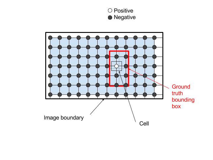
A position on the grid, that is the closest position to the center of one of the ground truth bounding boxes, is positive. Other positions are negative. The cell in the figure below gathers all possible position for the center of a ground truth box to activate the network output as positive:

So, let us keep these circles as a representation of the net outputs, and for the grid, rather than displaying a grid of the outputs, let us use this grid to separate the zones for which any ground truth box center will make these positions as positive. For that purpose, I can simply shift the grid back by half a stride:

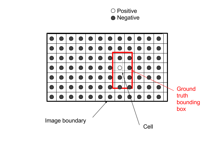
Note that in a more general case, a position could be considered as positive for bigger or smaller cells than the network stride, and in such a case, it would not be possible to see the separations between the region of attraction of each position in a grid.

A regressor rather than a classifier

For every positive position, the network predicts a regression on the bounding box precise position and dimension.

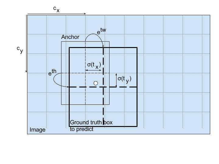
In the second version of Yolo, these predictions are relative to the grid position and anchor size (instead of the full image) as in the Faster-RCNN models for better performance:

\[b_x = \sigma(t_x) + c_x\] \[b_y = \sigma(t_y) + c_y\] \[b_w = p_w \ e^{t_w}\] \[b_h = p_h \ e^{t_h}\]

where \((c_x, c_y)\) are the grid cell coordinates and \((p_w, p_h)\) the anchor dimensions.

Confidence

Once the bounding box regressor is trained, the model is also trained to predict a confidence score on the final predicted bounding box with the above regressor.

The natural confidence score value is:

for a positive position, the intersection over union (IOU) of the predicted box with the ground truth
for a negative position, zero.

In the Yolo papers, confidence is trained jointly with the position/dimension regressor, which can cause model instability. To avoid this, they weighted the position/dimension regressor loss 5 times the confidence regressor loss.

Anchors or prediction specialization

Yolo V1 and V2 predict B regressions for B bounding boxes. Only one of the B regressors is trained at each positive position, the one that predicts a box that is closest to the ground truth box, so that there is a reinforcement of this predictor, and a specialization of each regressor.

In Yolo V2, this specialization is ‘assisted’ with predefined anchors as in Faster-RCNN. The predefined anchors are chosen to be as representative as possible of the ground truth boxes, with the following K-means clustering algorithm to define them:

all ground-truth bounding boxes are centered on (0,0)
the algorithm initiates 5 centroïds by drawing randomly 5 of the ground-truth bounding boxes
then, the following two steps are alternated:
- each ground truth box is assigned to one of the centroïd, using as distance measure the IOU, in order to get 5 clusters or groups of ground-truth bouding boxes
- new centroïds are computed by taking the box inside each cluster that minimizes the mean IOU with all other boxes inside the cluster

All together

For each specialization, in Yolo V2, the class probabilities of the object inside the box is trained to be predicted, as the confidence score, but conditionally on positive positions.

Putting it all together for an example of 5 anchors, 20 object classes, the output of the network at each position can be decomposed into 3 parts:

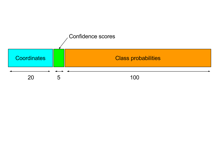
For all outputs except the relative width and height, the outputs are followed by the logistic activation function or sigmoid, so that the final outputs fall between 0 and 1. For the relative width and height, the activation is the exponential function.

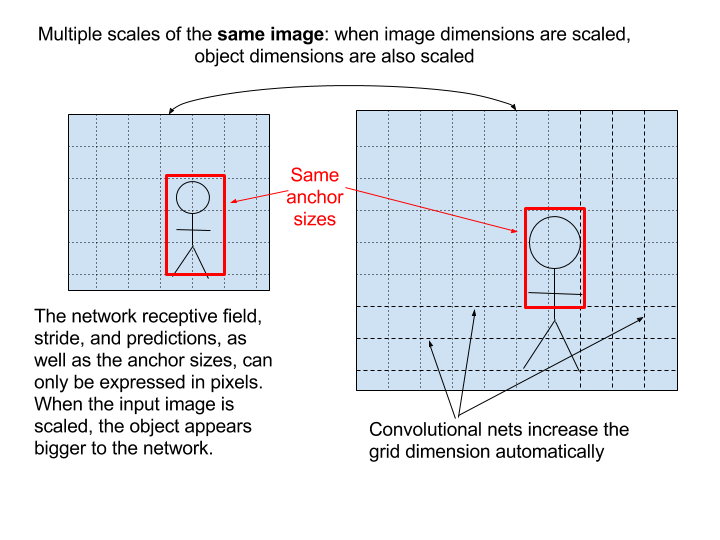
Multi-scale training

The multi-scale training consists in augmenting the dataset so that objects will be at multiple scales. Since a neural network works with pixels, resizing the images in the dataset at multiple sizes simply enable to simulate objects of multiple scales.

Note that some neural network implementations resize all images to a given size, let’s say 500x500, as a kind of first layer in the neural network. First, this automatic resizing step cancels the multi-scale training in the dataset. Second, there is also a problem with ratio since the network in this case will learn to deal with square images only: either part of the input image is discarded (crop), or the ratio is not preserved, which is suboptimal in both cases.

The best way to deal with images of multiple sizes is to let the convolutions do the job: convolutions will automatically add more cells along the width and height dimensions to deal with images of different sizes and ratios. The only thing that you need to remind of is that a neural network works with pixels, that means each output value in the grid is a function of the pixels inside the receptive field, a function of the object resolution and not a function of the image width and height.

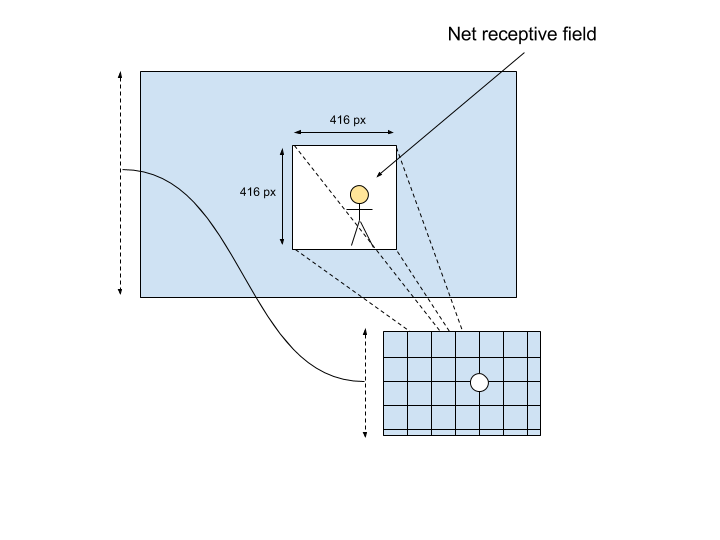
The global image width/height impacts the number of cells in the grid, vertically and horizontally. Locally, each stack of convolutions and max-pooling layers composing the net uses the pixel patch in the receptive field to compute the prediction and ignores the total number of cells and the global image width/height.

This leads to the following point: anchor sizes can only be expressed in pixels as well. In order to allow multi-scale training, anchors sizes will never be relative to the input image width or height, since the objective of multi-scale training is to modify the ratio between the input dimensions and anchor sizes.

In Yolo implementations, these sizes are given with respect to the grid size, which is a fixed number of pixels as well (the network stride, ie 32 pixels):

Yolo anchors for VOC dataset:

3221, 1.73145
19275, 4.00944
05587, 8.09892
47112, 4.84053
2364, 10.0071

Well done!