UPDATE! : my Fast Image Annotation Tool for Spatial Transformer supervised training has just been released ! Have a look !

Spatial Transformer Networks

Spatial Transformer Networks (SPN) is a network invented by Max Jaderberg, Karen Simonyan, Andrew Zisserman, Koray Kavukcuoglu at Google DeepMind artificial intelligence lab in London.

The use of a SPN is

• to improve classification

• to subsample an input

• to learn subparts of objects

• to locate objects in an image without supervision

SPN predicts the coefficients of an affine transformation :

The second important thing about SPN is that it is trainable : to predict the transformation, SPN can retropropagate gradients inside its own layers.

Lastly, SPN can also retropropagate gradients to the image or previous layer it operates on, so they can be placed anywhere inside a neural net.

The maths

If \((x,y)\) are normalized coordinates, \((x,y) \in [-1,1] \times [-1,1]\), an affine transformation is given by a matrix multiplication :

A simple translation by \((t_x,t_y)\) would be

An isotropic scaling by a factor s would be

For a clockwise rotation of angle \(\alpha\)

The global case for a clockwise rotation of angle \(\alpha\), a scaling by a factor s, and a translation of the center of \((t_x,t_y)\), in any order, would be

So, I have an easily differentiable function \(\tau\) (multiplications and additions) to get the corresponding position in the input image for a given position in the output image :

and, to compute the pixel value in our output image of the SPN, I can just take the value in the input image at the right place

But usually, \(\tau ( x_{out}, y_{out} )\) is not an integer value (on the image grid), so we need to interpolate it :

There exists many ways to interpolate : nearest-neighbor, bilinear, bicubic, … (have a look at OpenCV and Photoshop interpolation options as an example), but the best is to use a differentiable one. For example, the bilinear interpolation function for any continuous position in the input image \((X,Y) \in [0,M] \times [0,N]\)

which is easily differentiable

• in position \(\frac{\partial bilinear}{\partial X }\) which enables to learn the \(\theta\) parameters because

  \[I_{out}( x_{out}, y_{out} ) = bilinear( \tau_{\theta} ( x_{out}, y_{out} ), I_{in} )\] \[\frac{\partial I_{out}}{\partial \theta } = \frac{\partial bilinear}{\partial X } \times \frac{\partial \tau_{x}}{\partial \theta }\]

• in image \(\frac{\partial bilinear}{\partial I }\) which enables to put the SPN on top of other SPN or other layers such as convolutions, and retropropagate the gradients to them (set to_compute_dU option in layer params to true).

Now we have all the maths !

Spatial Transformer Networks in Caffe

I updated Caffe with Carey Mo implementation :

git clone https://github.com/christopher5106/last_caffe_with_stn.git

Compile it as you compile Caffe usually (following my tutorial on Mac OS or Ubuntu ).

Play with the theta parameters

Let’s create our first SPN to see how it works. Let’s fix a zoom factor of 2, and leave the possibility of a translation only :

For that, let’s write a st_train.prototxt file :

name: "stn"
input: "data"
input_shape {
  dim: 1
  dim: 3
  dim: 227
  dim: 227
}
input: "theta"
input_shape {
  dim: 1
  dim: 2
}
layer {
  name: "st_1"
  type: "SpatialTransformer"
  bottom: "data"
  bottom: "theta"
  top: "transformed"
  st_param {
    to_compute_dU: false
    theta_1_1: 0.5
    theta_1_2: 0.0
    theta_2_1: 0.0
    theta_2_2: 0.5
  }
}

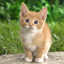
Lets load our cat :

caffe.set_mode_gpu()
net = caffe.Net('sp_train.prototxt',caffe.TEST)
image = caffe.io.load_image("cat-227.jpg")
plt.imshow(image)

[(‘data’, (1, 3, 227, 227)), (‘theta’, (1, 2)), (‘transformed’, (1, 3, 227, 227))]

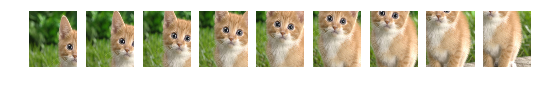
and translate in diagonal :

transformer = caffe.io.Transformer({'data': net.blobs['data'].data.shape})
transformer.set_transpose('data', (2,0,1))  # move image channels to outermost dimension
#transformer.set_mean('data', mu)            # subtract the dataset-mean value in each channel
transformer.set_raw_scale('data', 255)      # rescale from [0, 1] to [0, 255]
transformer.set_channel_swap('data', (2,1,0))  # swap channels from RGB to BGR
transformed_image = transformer.preprocess('data', image)
net.blobs['data'].data[...] = transformed_image
for i in range(9):
    plt.subplot(1,10,i+2)
    theta_tt = -0.5 + 0.1 * float(i)
    net.blobs['theta'].data[...] = (theta_tt, theta_tt)
    output = net.forward()
    plt.imshow(transformer.deprocess('data',output['transformed']))
    plt.axis('off')

Test on the MNIST cluttered database

Let’s create a folder of MNIST cluttered images :

git clone https://github.com/christopher5106/mnist-cluttered
cd mnist-cluttered
luajit download_mnist.lua
mkdir -p {0..9}
luajit save_to_file.lua
for i in {0..9}; do for p in /home/ubuntu/mnist-cluttered/$i/*; do echo $p $i >> mnist.txt; done ; done

And train with a stn protobuf file, the bias init, and solver file.

./build/tools/caffe.bin train -solver=stn_solver.prototxt

OK, great, it works.

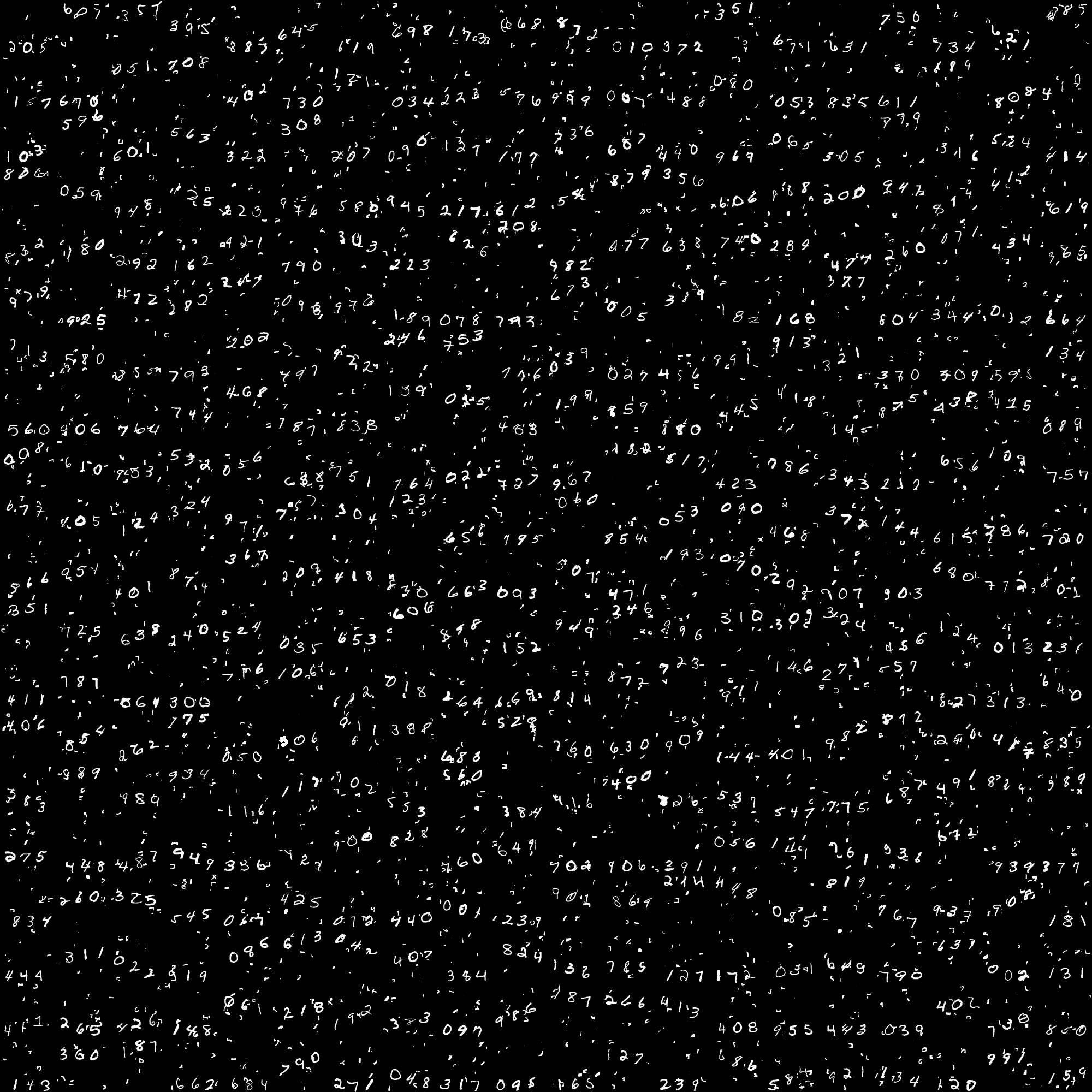
Supervised learning of the affine transformation for document orientation / localization

Given a dataset of 2000 annotated documents, I’m using my extraction tool to create 50 000 annotated documents by adding a random rotation noise of +/- 180 degrees.

I train a GoogLeNet to predict the \(\theta\) parameters.

Once trained, let’s have a look at our predictions :

Unsupervised learning of the spatial transformation to center the character during reading

Let’s add our SPN in front of our MNIST neural net for which we had a 98% success rate on plate letter identification and train it on a more difficult database of digits, with clutter and noise in translation, on which I only have 95% of good detection.

I just need to change the last innerproduct layer to predict the 6 coordinates of \(\theta\) :

layer {
  name: "loc_reg"
  type: "InnerProduct"
  bottom: "loc_ip1"
  top: "theta"
  inner_product_param {
    num_output: 6
    weight_filler {
      type: "constant"
      value: 0
    }
    bias_filler {
      type: "file"
      file: "bias_init.txt"
    }
  }
}

with bias initialized at 1 0 0 0 1 0.

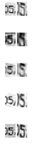
The SPN helps stabilize the detection, by centering the image on the digit before the recognition. The rate comes back to 98%.

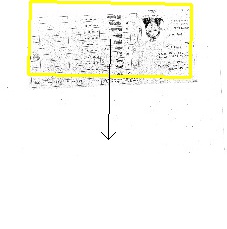
Unsupervised learning for document localization

Let’s try with 2 GoogLeNet, one in the SPN to predict the affine transformation, and the other one after for object classification.

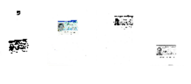
The SPN repositions the document around the same place roughly :

Spatial tranformer networks in Tensorflow

Have a look at Tensorflow implementation.

Rotation-only spatial transformer networks

Instead of learning the \(\theta\) parameter, which we cannot constrain to a rotation, it’s possible to learn an \(\beta = \alpha / 180 \in [-1,1]\) parameter :

and replacing with

where

Well done!