It is so easy to train a recurrent network with Caffe.

Install

Let’s compile Caffe with LSTM layers, which are a kind of recurrent neural nets, with good memory capacity.

For compilation help, have a look at my tutorials on Mac OS or Linux Ubuntu.

In a python shell, load Caffe and set your computing mode, CPU or GPU :

import sys
sys.path.insert(0, 'python')
import caffe
caffe.set_mode_cpu()

Single LSTM

Let’s create a lstm.prototxt defining a LSTM layer with 15 cells, the number of cells defining the memory capacity of the net, and an InnerProduct Layer to output a prediction :

name: "LSTM"
input: "data"
input_shape { dim: 320 dim: 1 }
input: "clip"
input_shape { dim: 320 dim: 1 }
input: "label"
input_shape { dim: 320 dim: 1 }
layer {
  name: "Silence"
  type: "Silence"
  bottom: "label"
  include: { phase: TEST }
}
layer {
  name: "lstm1"
  type: "Lstm"
  bottom: "data"
  bottom: "clip"
  top: "lstm1"

  lstm_param {
    num_output: 15
    clipping_threshold: 0.1
    weight_filler {
      type: "gaussian"
      std: 0.1
    }
    bias_filler {
      type: "constant"
    }
  }
}
layer {
  name: "ip1"
  type: "InnerProduct"
  bottom: "lstm1"
  top: "ip1"

  inner_product_param {
    num_output: 1
    weight_filler {
      type: "gaussian"
      std: 0.1
    }
    bias_filler {
      type: "constant"
    }
  }
}
layer {
  name: "loss"
  type: "EuclideanLoss"
  bottom: "ip1"
  bottom: "label"
  top: "loss"
  include: { phase: TRAIN }
}

and its solver :

net: "lstm.prototxt"
test_iter: 1
test_interval: 2000000
base_lr: 0.0001
momentum: 0.95
lr_policy: "fixed"
display: 200
max_iter: 100000
solver_mode: CPU
average_loss: 200
#debug_info: true

LSTM params are three matrices defining for the 4 computations of input gate, forget gate, output gate and hidden state candidate :

U, the input-to-hidden weights : 4 x 15 x 1
W, the hidden-to-hidden weights : 4 x 15 x 15
b, the bias : 4 x 15 x 1

\[i = \sigma( x_t U^i + s_{t-1} W^i + b^i)\] \[f = \sigma( x_t U^f + s_{t-1} W^f + b^f)\] \[o = \sigma( x_t U^o + s_{t-1} W^o + b^o)\] \[g = \tanh( x_t U^g + s_{t-1} W^g + b^g )\] \[c_t = c_{t-1} \circ f + g \circ i\] \[s_t = \tanh(c_t) \circ o\]

The LSTM layer contains blobs of data :

a memory cell of size H, previous c_0 and next c_T
hidden activation values of size H, previous h_0 and next h_T

for each step (\(T \times N\)).

As input, of the LSTM :

data, of dimension \(T \times N \times I\), where I is the dimensionality of the data (1 in our example) at each step in the sequence, \(T \times N\) the sequence length and N the batch size. The constraint is that the data size has to be a multiple of batch size N.
clip, of dimension \(T \times N\). If clip=0, hidden state and memory cell will be initialiazed to zero. If not, their previous value will be used.
label, the target to predict at each step.

And load the net in Python :

solver = caffe.SGDSolver('solver.prototxt')

Set the bias to the forget gate to 5.0 as explained in the clockwork RNN paper

solver.net.params['lstm1'][2].data[15:30]=5

Let’s create a data composed of sinusoids and cosinusoids :

import numpy as np
a = np.arange(0,32,0.01)
d = 0.5*np.sin(2*a) - 0.05 * np.cos( 17*a + 0.8  ) + 0.05 * np.sin( 25 * a + 10 ) - 0.02 * np.cos( 45 * a + 0.3)
d = d / max(np.max(d), -np.min(d))
d = d - np.mean(d)

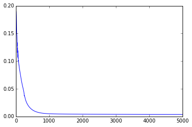
Let’s train :

niter=5000
train_loss = np.zeros(niter)
solver.net.params['lstm1'][2].data[15:30]=5
solver.net.blobs['clip'].data[...] = 1
for i in range(niter) :
    seq_idx = i % (len(d) / 320)
    solver.net.blobs['clip'].data[0] = seq_idx > 0
    solver.net.blobs['label'].data[:,0] = d[ seq_idx * 320 : (seq_idx+1) * 320 ]
    solver.step(1)
    train_loss[i] = solver.net.blobs['loss'].data

and plot the results :

import matplotlib.pyplot as plt
%matplotlib inline
plt.plot(np.arange(niter), train_loss)

Let’s test the result :

solver.test_nets[0].blobs['data'].reshape(2,1)
solver.test_nets[0].blobs['clip'].reshape(2,1)
solver.test_nets[0].reshape()
solver.test_nets[0].blobs['clip'].data[...] = 1
preds = np.zeros(len(d))
for i in range(len(d)):
    solver.test_nets[0].blobs['clip'].data[0] = i > 0
    preds[i] =  solver.test_nets[0].forward()['ip1'][0][0]

and plot :

plt.plot(np.arange(len(d)), preds)
plt.plot(np.arange(len(d)), d)
plt.show()

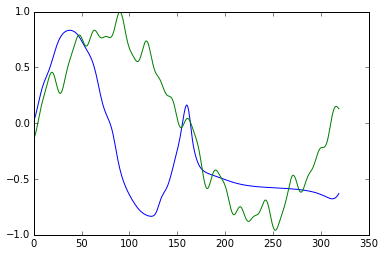
We have to put more memory, and stack the LSTM, to get better results!

Repeat layer

As in Recurrent Spatial Transformer Networks, it can be very usefull to have a Repeat Layer to repeat the value of an image vector into the different steps of the RNN.

This kind of layer can be useful to transfer less data to the GPU, and go faster since transfer time are the bottleneck.

Let’s see in practice how it works, and create a repeat.prototxt

name: "Repeat"
input: "data"
input_shape { dim: 10 dim: 1 }
layer {
  name: "loss_repeat"
  type: "Repeat"
  bottom: "data"
  top: "repeated"
  propagate_down: 1
  repeat_param {
    num_repeats: 32
  }
}

If we set for example for num_repeats=3,

\[W = \left[ \begin{array}{ccc} 1 & 0 & 0 \\ 0 & 1 & 0 \\ 0 & 0 & 1 \\ 1 & 0 & 0 \\ 0 & 1 & 0 \\ 0 & 0 & 1 \\ 1 & 0 & 0 \\ 0 & 1 & 0 \\ 0 & 0 & 1 \end{array} \right]\]

then the forward pass is a simple matrix multiplication :

\[V_{n,j} = \Sigma_{i=0}^{num\_repeats * K} U_{n,i} w_{j,i}\] \[V = U \times W^T\]

The backward pass

\[\delta U_{n,i} = \Sigma_{j=0}^K \delta V_{n,j} w_{j,i}\] \[\delta U = \delta V \times W\]

Let’s test it :

import sys
sys.path.insert(0, 'python')
import caffe
caffe.set_mode_cpu()
net = caffe.Net('repeat.prototxt',caffe.TEST)
import numpy as np
net.blobs['data'].data[...]=np.arange(0,10,1).reshape(10,1)
print "input", net.blobs['data'].data[5]
out = net.forward()["repeated"]
print "output shape", out.shape
print "output", out

Well done!