Here is my course of deep learning in 5 days only! You might first check Course 0: deep learning!, Course 1: program deep learning! and course 2: build deep learning networks! if you have not read them.

In this article, I develop techniques for natural language. Tasks include text classification (finding the sentiment, positive or negative, the language, …), segmentation (POS taging, Named Entities extraction ,…), translation, … as in computer vision.

But, while computer vision deals with continuous (pixel values) and fixed-length inputs (images, usually resized or cropped to a fixed dimension), natural language consists of variable-length sequences (words, sentences, paragraphs, documents) of discrete inputs, either characters or words, belonging to a fixed size dictionary (the alphabet or the vocabulary respectively), depending if we work at character level or word level.

There are two challenges to overcome :

• transforming discrete inputs into continuous representations or vectors

• transforming variable-length sequences into a fixed-length representations

The dictionary of symbols

Texts are sequences of characters or words, depending if we word at character level or word level. It is possible to work at both levels and concatenate the representations at higher level in the neural network. The dictionary is a fixed-size list of symbols found in the input data: at character level, we call it an alphabet, while at word level it is usually called a vocabulary. While the words incorporate a semantic meaning, the vocabulary has to be limited to a few tens thousands entries, so many out-of-vocabulary tokens cannot be represented.

There exists a better encoding for natural language, the Byte-Pair-Encoding (BPE), a compression algorithm that iteratively replaces the most frequent pairs of symbols in sequences by a new symbol: initially, the symbol dictionary is composed of all characters plus the ‘space’ or ‘end-of-word’ symbol, then recursively count each pair of symbols (without crossing word boundaries) and replace the most frequent pair by a new symbol.

For example, if (‘T’, ‘H’) is the most frequent pair of symbols, we replace all instances of the pair by the new symbol ‘TH’. Later on, if (‘TH’, ‘E’) is most frequent pair, we create a new symbol ‘THE’. The process stops when the desired target size for the dictionary has been achieved. At the end, the symbols composing the dictionary are essentially characters, bigrams, trigrams, as well as most common words or word parts.

The advantage of BPE is to be capable of open-vocabulary through a fixed-size vocabulary though, while still working at a coarser level than characters. In particular, names, compounds, loanwords which do not belong to a language word vocabulary can still be represented by BPE. A second advantage is that the BPE preprocessing works for all languages.

In translation, better results are achieved by joint BPE, encoding both the target and source languages with the same dictionary of encoding. For languages using a different alphabets, characters are transliterated from one alphabet to the other. This helps in particular to copy Named Entities which do not belong to a dictionary.

Last, it is possible to relax the greedy and deterministic symbol replacement of BPE, by using a unigram language model that assumes that each symbol is an unobserved latent variable of the sequence and occurs independently in the sequence. Given this assumption, the probability of a sequence of symbols \((x_1, ..., x_M)\) is given by :

and the probability of a sentence or text S to occur is given by the sum of probabilities of each encodings:

So it is possible to compute a dictionary of the desired size that maximizes (locally) the likelihood by an iterative algorithm starting from a huge dictionary of most frequent substring, estimating the expectation as in the EM algorithm, and removing the subwords with less impact on the likelihood. Also, multiple decodings into a sequence of symbols are possible for a text and the model gives each of them a probability. At training time, it is possible to sample a decoding of the input given the symbol distribution. At inference, it is possible to compute the predictions using multiple decodings, and choose the most confident prediction. Such a technique, called subword regularization, augments the training data stochastically and improves accuracy and robustness in natural language tasks.

Have a look at SentencePiece. Note that ‘space’ character is treated as a symbol and pretokenization of the sequences is not necessary.

Distributed representations of the symbols

Now we have a dictionary, each text block can be represented by a sequence of token ids. Such a representation is discrete and does not encode the semantic meaning of the token. In order to do so, we associate each token with a vector of dimension d to be learned. All tokens are represented by an embedding matrix

when V is the size of the dictionary.

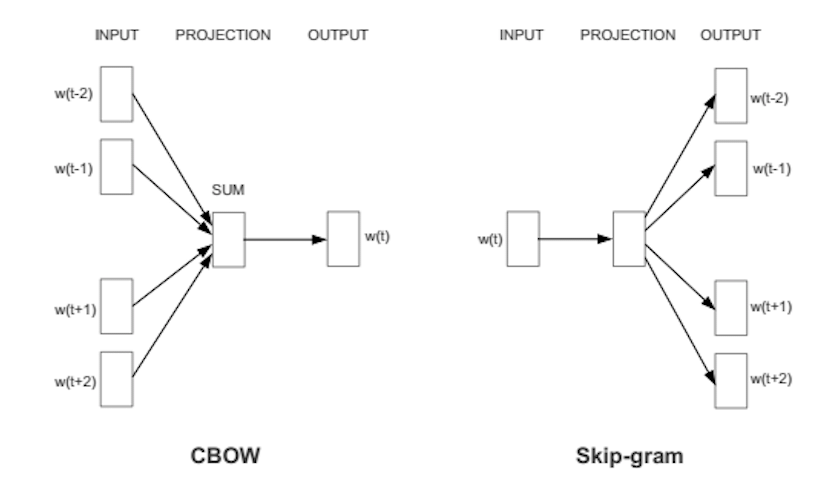
Two architectures were proposed :

• the Continuous Bag-of-Words (CBOW) to predict the current word based on the context, and

• the Continuous Skip-gram to predict the context words based on the current word,

with a simple feedforward model :

where X and X’ \(\in \mathbb{R}^V\) are the one-hot encoding vector of the input and output words (with 1 if the word occur in the input and output respectively), W and \(\hat{W}\) are the input and output embedding matrices.

One of the difficulty is due to the size of the output, equal to the size of the dictionary. Some solutions have been proposed: hierarchical softmax with Huffman binary trees, avoiding normalization during training, or stochastic negative mining (Noise Contrastive Estimation and Negative Sampling with a sampling distribution avoiding frequent words).

Once trained, such weights W can be refined on high level tasks such as similarity prediction, translation, etc. They can be found under the names word2vec, GloVe, Paragram-SL999, …, and used to initialize the first layer of neural networks. In any application, they can be either fixed or trained further.

The next step is to address representations for blocks of text, ie sentences, paragraphs or documents. Before that, I first present new layers initially designed for natural language.

Recurrent neural networks (RNN)

A recurrent network can be defined as a feedforward (non recurrent) network with two inputs, the input at time step t and previous hidden state \(h_{t-1}\), to produce a new state at time t, \(h_t\).

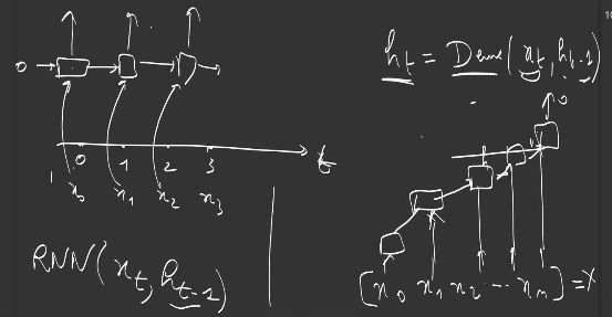
Recurrent models have been used in the past to transform a sequence of vectors (the learned word representations seen in previous section) into one vector, reducing variable-length representation into a fixed-length representation. Now they are outdated and been replaced by transformers.

It is very frequent to find some BiLSTM, where LSTM is a type of RNN applied two times to the sequence, in natural and reverse orders, both outputs being concatenated.

Attention, self-attention and Transformer

The attention mechanism takes as input a query, an input sequence transformed into keys and values . It consists in finding the relevant entries in the input sequence, given a query represented by a (512,) vector as presented in the following figure:

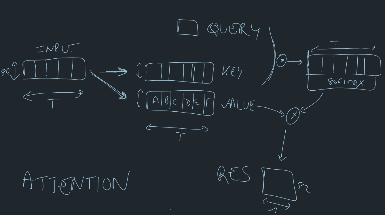
The query is compared with keys, a matrix of dimension (T, 512) for 1 sample, or (B, T, 512) for a batch of samples, and the dot product is used as comparison operator. Be careful to normalize output of the scalar product by \(\frac{1}{\sqrt{d}}\), where d is the dimensionality of the data, in order to keep variance 1.

The result is passed through a softmax layer in order to get a probability \(p_t\) for each of the T positions in the sequence. The values, another matrix of dimension (T, 512) or (B, T, 512), is used to computed the final result, of dimension (512,):

Self-attention is when each position of the input sequence is used a query. The output is of shape (T, 512), the same length as the input, T. 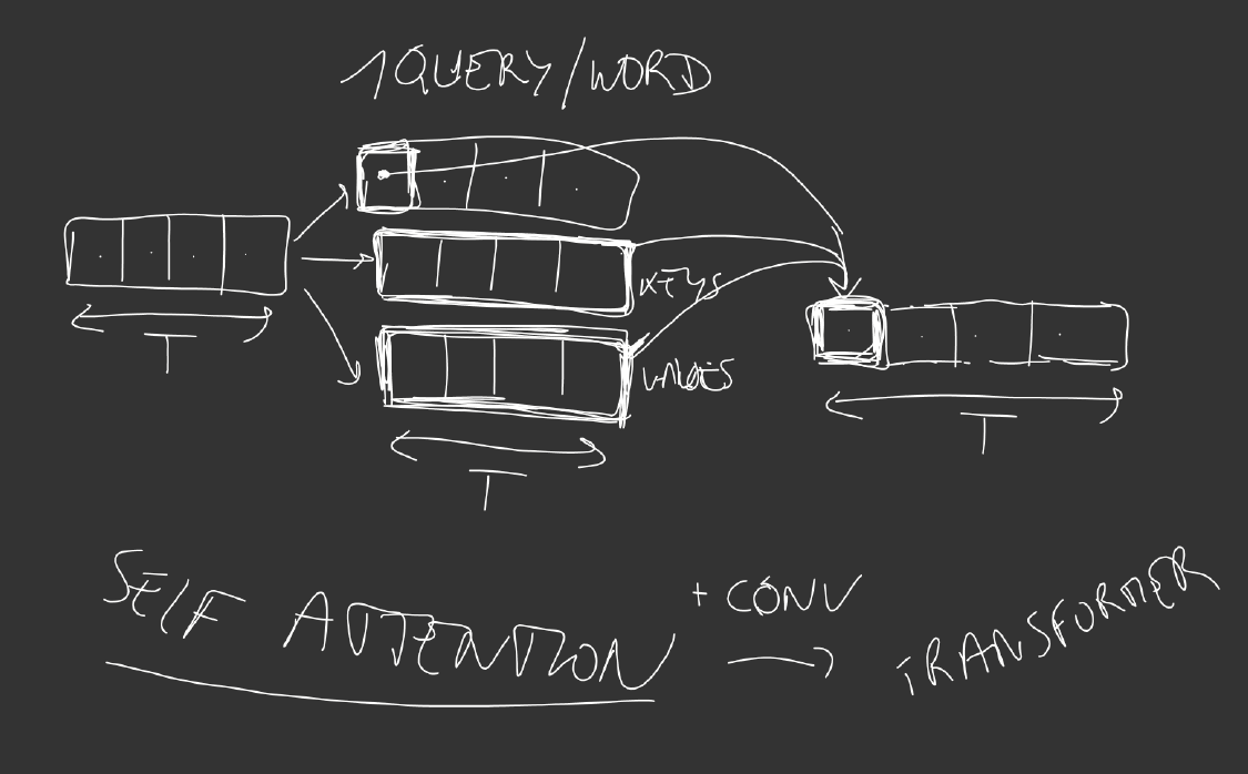Such a mechanism enables to take into account each word of the context to compute the representation of a word.

The Transformer is an architecture using convolutions and self attention, described here.

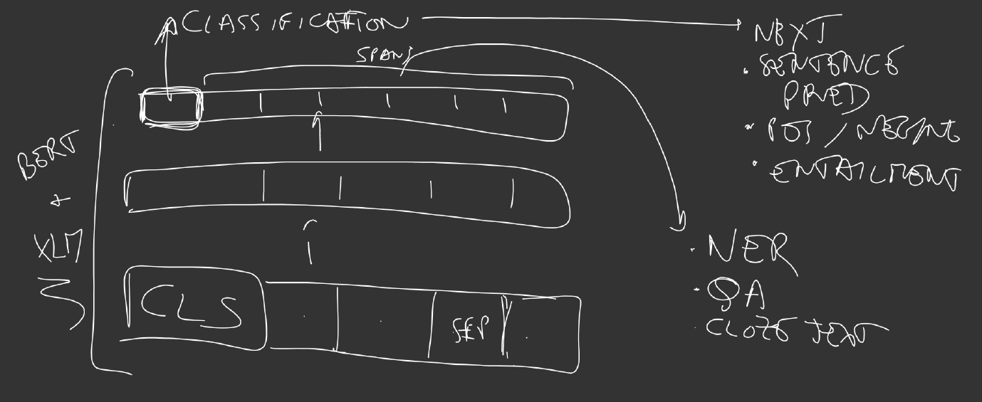
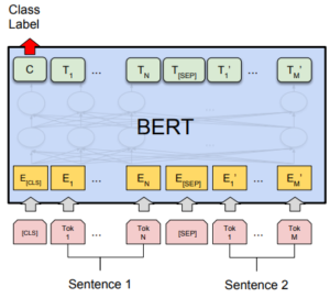
For classification tasks, such as sentiment analysis, the output at the start token (or first token) is taken to represent the sequence and be further processed by a simple classifier. For segmentation tasks, such as question answering (QA) or named entity recognition (NER), all other outputs are used as input to the classifier:

In translation, both encoder and decoder incorporate a Transformer:

The self-attention enables computation efficiency and reduces the depth that accounts in the vanishing gradient problem:

Sentences, paragraphs or documents

There is a long history of attempts to represent block of texts.

The first idea, the simplest one, was to compute the average of the word representations. First results were convincing, and improved by the introduction of a weighted average, reweighting each word vector by the smooth inverse frequency $$ \frac{a}{a+IDF}, so that very frequent words, stop words, are less important than rare words.

Other techniques include the computation of a paragraph vector which can be considered as a special embedding, as if one special word has been added to each sentence to supplement the word embeddings and account for the semantic information in the paragraph. While initial idea required lot’s of gradient descents during inference, new techniques, such as CoVe, are computed directly by a forward pass of a two-layer BiLSTM on the sentence. The output of the trained BiLSTM at the word position is concatenated with the classical word representations (GloVe for example).

While CoVe biLSTM is trained on a translation task, Elmo’s stack of BiLSTM is trained on monolingual language model (LM) task, and the output of each BiLSTM layer is taken into the concatenation with the GloVe word representations.

The current state of the art for deep contextualized representation is BERT. Instead of BiLSTM, it uses state-of-art Transformer, and masks the words to predict at the output. This way, Transformers use all other words to perform the predictions, while LSTM could only use the previous ones (or the next ones for the reverse order). In the meantime, BERT is trained on two sentences, either consecutive in the text or randomly chosen, to predict also if sentence B follows sentence A. Last, a multilingual BERT model trained on 104 languages is just less 3% off the single-language model.

By simply adding a linear layer on top of BERT’s output, state-of-the-art has been achieved on Squad Question Answering dataset, SWAG dataset, and GLUE datasets, demonstrating that these embeddings capture well the semantics of blocks of text.

BERT has a cross-lingual version, trained with translation parallel data to build representations independent of language:

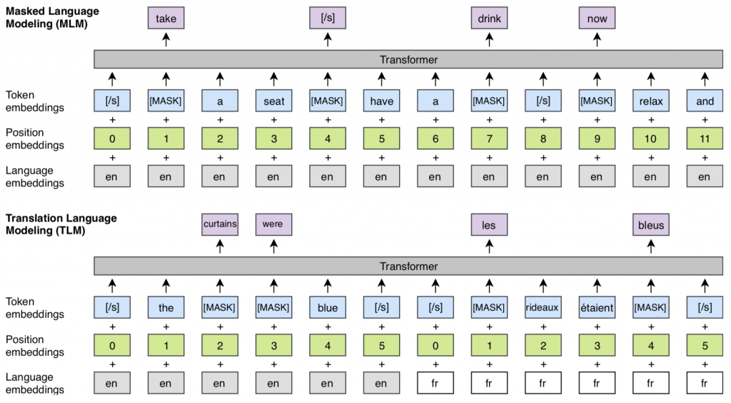
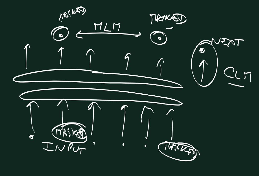
The training of BERT and XLM embedding is performed with one of the following losses:

• the causal language model (CLM): predicting the next word in the sentence
• the masked language model (MLM): predicting the randomly masked or replaced words.
• the translation language model (TLM) : it is like a CLM but for a sequence consisting of 2 sentences in 2 different languages, translation of each other, with reset position embeddings so that the model can use either both sentences indifferently to predict the masked or replaced words, leading to aligned representations for different languages.

Metrics for translation

Models are trained to maximize the log likelihood, but this does not give any idea of the final quality of the model. Since human evaluations is costly and long, metrics have been developped that correlates well with human judgments, on a given set of possible translations (reference translations) for the task of translation for example.

The ChrF3 is one of them, the most simple one, is the F3-score for the character n-grams. The best correlations are obtained with \(n=6\). The ChrF3 has a recall bias.

Another metric, BLUE, has a precision bias. It is the precision for the character n-grams, where the count for each n-gram matches is clipped, not to be bigger than the number of n-grams in the reference translation, in order to penalize translation systems that generate a same word multiple times. The metric can be case-sensitive, in order to take into account the Named Entities for example.

ROUGE-n is the recall equivalent metric.

There exists metrics on words (called unigrams) also, such as

• WER (Word Error Rate), the Levenstein distance at word level.

• METEOR, the ChrF3 equivalent at word level, reweighted by a non-alignment penalty.

Next course ! encoder decoder architectures, generative networks, and adversarial training !

Well done!