Tensorflow : a deep learning library by Google, let's give it a try
TensorFlow comes as a library such as other deep learning libraries, Caffe, Theano, or Torch. I’ve already written a lot on Caffe before.
This article is a global overview. To learn in detail symbolic computing, have a look at my new tutorial to understand Tensorflow and Theano symbolic computing.
The main advantage of Tensorflow
Such as Caffe, TensorFlow comes with an API in both Python and C++ languages.
Python is great for the tasks of experimenting and learning the parameters. These tasks may require tons of data manipulation before you get to the correct prediction model. Remember that 80% of the job of the data scientist is to prepare data, first clean it, then find the correct representation from which a model can learn. Learning comes last, as 20% of the work.
Tensorflow enables GPU computation which is also a very useful feature when it comes to learning, which requires usually from a few tens minutes to a few tens hours : learning time will be divided by 5 to 50 on GPU which makes playing with hyperparameters of the model very convenient.
Lastly, when the model has been learned, it has to be deployed in production apps, and usually, speed and optimizations become more important : the C++ API is the expected first choice for this purpose.
Tensorflow comes with Tensorboard, which looks like the DIGITS interface from NVIDIA (see my tutorial on Mac or on Ubuntu), but with much more flexibility on the events to display in the reports :
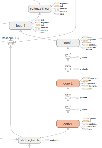
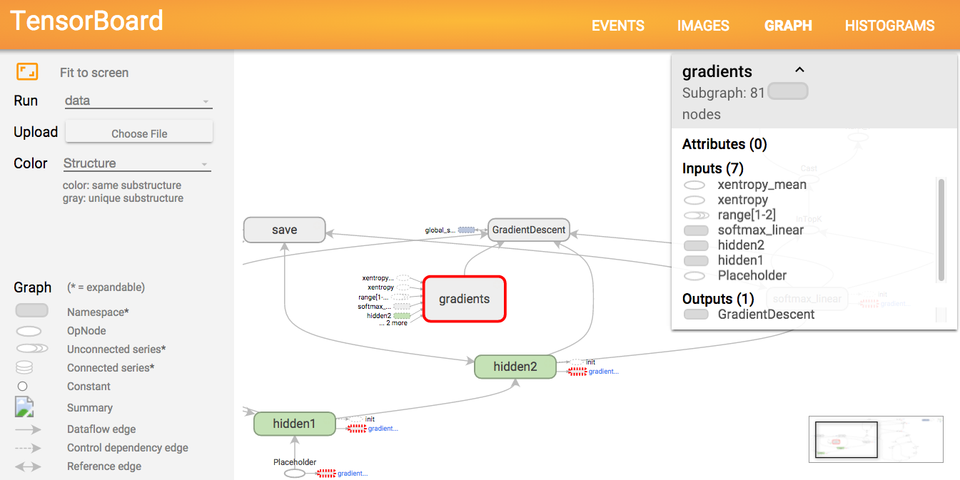
and a graph visualization tool, that works like our python python/draw_net.py command in Caffe, but with different informations (see tutorial)
I would say that Tensorflow brings nothing really new, but the main advantage is that everything is in one place, and easy to install, which is very nice.
Such as Theano, TensorFlow has taken the bet of symbolic computation which brings lots of flexibility to layer definitions and simplifies coding with automatic differentiation of equations for the back propagation (gradient descent). This enables creation of networks directly and integrally from the Python code (without having to write a ‘NetSpec’ interface such as in Caffe).
TensorBoard brings what DIGITS brings to Caffe and other deep learning libraries. Graph visualization brings informations about the operations that will occur in the processing, that no other library proposes.
A “best-in-class” work, but it can still be challenging to understand the real added-value compared to other tools.
A contrario, I would see these main drawbacks :
-
if some needed operations are not available in the library, I cannot imagine how complex it can be to add them…
-
TensorBoard does not simplify understanding of the network, is too much thorough, and display of some informations, such as the layer parameters, is missing compared to other tools … so I’m even more lost…
Caffe remains for me the main tool where R&D occurs, but I believe that Tensorflow will become greater and greater in the future.
Technical work done by Google is always very great.
Install
Let’s install Tensorflow on an iMac :
#pip install https://storage.googleapis.com/tensorflow/mac/tensorflow-0.5.0-py2-none-any.whl
pip install --upgrade https://storage.googleapis.com/tensorflow/mac/tensorflow-0.8.0-py2-none-any.whl
You will need protobuf version above 3.0 (otherwise you’ll get a TypeError: __init__() got an unexpected keyword argument 'syntax') :
brew uninstall protobuf
brew install --devel --build-from-source --with-python -vd protobuf
--devel options will enable to install version ‘protobuf>=3.0.0a3’.
How it works : a graph with inputs and variable data
As in Theano, the code you write is a symbolic abstraction : it describes operations, and operations belong to a connected graph, with inputs and outputs.
The first thing to do is to initialize variables in which to store the data for the net. Initialization is performed with the following operations :
# Create two variables.
weights = tf.Variable(tf.random_normal([784, 200], stddev=0.35),
                  name="weights")
biases = tf.Variable(tf.zeros([200]), name="biases")
...
# Add an op to initialize the variables.
init_op = tf.initialize_all_variables()

# Add ops to save and restore all the variables.
saver = tf.train.Saver()

# Later, when launching the model
with tf.Session() as sess:
# Run the init operation.
    sess.run(init_op)
    ...
# Use the model
    ...
# Save the variables to disk.
    save_path = saver.save(sess, "/tmp/model.ckpt")
    print "Model saved in file: ", save_path
A session is created, in which all variables are stored. The session enables communication with the processor (CPU, GPU).
Add neural network operations to the graph
Let’s run the softmax regression model example with a single linear layer :
git clone https://tensorflow.googlesource.com/tensorflow
cd tensorflow/tensorflow
python g3doc/tutorials/mnist/mnist_softmax.py
With mnist_softmax.py shown just below, consisting in adding symbolic operations on the data, tf.matmul (matrix multiplication), + (tensor addition), tf.nn.sofmax (softmax function), reduce_sum (sum) and minimize (minimization with GradientDescentOptimizer) :
import input_data
mnist = input_data.read_data_sets('MNIST_data', one_hot=True)
import tensorflow as tf
sess = tf.InteractiveSession()
x = tf.placeholder("float", shape=[None, 784])
y_ = tf.placeholder("float", shape=[None, 10])
W = tf.Variable(tf.zeros([784,10]))
b = tf.Variable(tf.zeros([10]))
sess.run(tf.initialize_all_variables())
y = tf.nn.softmax(tf.matmul(x,W) + b)
cross_entropy = -tf.reduce_sum(y_*tf.log(y))
train_step = tf.train.GradientDescentOptimizer(0.01).minimize(cross_entropy)
for i in range(1000):
  batch = mnist.train.next_batch(50)
  train_step.run(feed_dict={x: batch[0], y_: batch[1]})
correct_prediction = tf.equal(tf.argmax(y,1), tf.argmax(y_,1))
accuracy = tf.reduce_mean(tf.cast(correct_prediction, "float"))
print accuracy.eval(feed_dict={x: mnist.test.images, y_: mnist.test.labels})
Which gives an accuracy of ~0.91.
When it comes to the small convolutional network example :
import input_data
import tensorflow as tf
sess = tf.InteractiveSession()
mnist = input_data.read_data_sets('MNIST_data', one_hot=True)

def weight_variable(shape):
  initial = tf.truncated_normal(shape, stddev=0.1)
  return tf.Variable(initial)

def bias_variable(shape):
  initial = tf.constant(0.1, shape=shape)
  return tf.Variable(initial)
def conv2d(x, W):
  return tf.nn.conv2d(x, W, strides=[1, 1, 1, 1], padding='SAME')

def max_pool_2x2(x):
  return tf.nn.max_pool(x, ksize=[1, 2, 2, 1],
                        strides=[1, 2, 2, 1], padding='SAME')

x = tf.placeholder("float", shape=[None, 784])
y_ = tf.placeholder("float", shape=[None, 10])

W_conv1 = weight_variable([5, 5, 1, 32])
b_conv1 = bias_variable([32])
x_image = tf.reshape(x, [-1,28,28,1])
h_conv1 = tf.nn.relu(conv2d(x_image, W_conv1) + b_conv1)

h_pool1 = max_pool_2x2(h_conv1)

W_conv2 = weight_variable([5, 5, 32, 64])
b_conv2 = bias_variable([64])
h_conv2 = tf.nn.relu(conv2d(h_pool1, W_conv2) + b_conv2)

h_pool2 = max_pool_2x2(h_conv2)

W_fc1 = weight_variable([7 * 7 * 64, 1024])
b_fc1 = bias_variable([1024])
h_pool2_flat = tf.reshape(h_pool2, [-1, 7*7*64])
h_fc1 = tf.nn.relu(tf.matmul(h_pool2_flat, W_fc1) + b_fc1)

keep_prob = tf.placeholder("float")
h_fc1_drop = tf.nn.dropout(h_fc1, keep_prob)

W_fc2 = weight_variable([1024, 10])
b_fc2 = bias_variable([10])
y_conv=tf.nn.softmax(tf.matmul(h_fc1_drop, W_fc2) + b_fc2)

cross_entropy = -tf.reduce_sum(y_*tf.log(y_conv))

train_step = tf.train.AdamOptimizer(1e-4).minimize(cross_entropy)

correct_prediction = tf.equal(tf.argmax(y_conv,1), tf.argmax(y_,1))
accuracy = tf.reduce_mean(tf.cast(correct_prediction, "float"))

sess.run(tf.initialize_all_variables())

for i in range(20000):
  batch = mnist.train.next_batch(50)
  if i%100 == 0:
    train_accuracy = accuracy.eval(feed_dict={
        x:batch[0], y_: batch[1], keep_prob: 1.0})
    print "step %d, training accuracy %g"%(i, train_accuracy)
  train_step.run(feed_dict={x: batch[0], y_: batch[1], keep_prob: 0.5})

print "test accuracy %g"%accuracy.eval(feed_dict={
    x: mnist.test.images, y_: mnist.test.labels, keep_prob: 1.0})
the training accuracy consolidates above 0.98 after 8000 iterations, and the test accuracy closes at 0.9909 after 20 000 iterations.
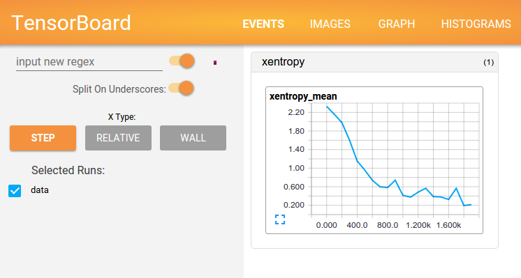
Let’s try the feed forward neural network defined in fully_connected_feed.py :
#first launch Tensorboard to see the results in http://localhost:6006/
#be careful to write full path because it checks path existence
tensorboard --logdir=/Users/christopherbourez/examples/tensorflow/tensorflow/data
#i had to edit fully_connected_feed.py to replace tensorflow.g3doc.tutorials.mnist by g3doc.tutorials.mnist
python g3doc/tutorials/mnist/fully_connected_feed.py
Which gives the following results
Training Data Eval:
Num examples: 55000  Num correct: 49365  Precision @ 1: 0.8975
Validation Data Eval:
Num examples: 5000  Num correct: 4530  Precision @ 1: 0.9060
Test Data Eval:
Num examples: 10000  Num correct: 9027  Precision @ 1: 0.9027
And in Tensorboard (at http://localhost:6006/)
Have a look at my tutorial about symbolic programming in Tensorflow or Theano.
Well done!