Here is my course of deep learning in 5 days only!

You might first check Course 0: deep learning! and Course 1: program deep learning! if you have not read them.

Common layers for deep learning

After the Dense layer seen in Courses 0 and 1, also commonly called fully connected (FC) or Linear layers, let’s go further with new layer.

Convolutions

Convolution layers are locally linear layers, defined by a kernel consisting of weights working on a local zone of the input.

On a 1-dimensional input, a 1D-convolution of kernel k=3 is defined by 3 weights \(w_1, w_2, w_3\). The first output is computed:

Then next output is the result of shifting the previous computation by one:

And

If the input is of length \(l_I\), a 1D-convolution of kernel 3 can only produce values for

positions, hence \((n -2)\) positions in the case of kernel 3.

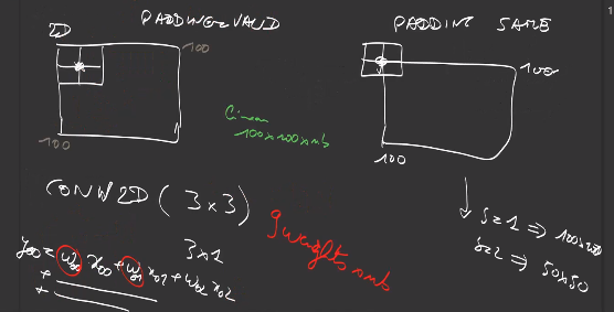
It is also possible to define the stride of the convolution, for example with stride 2, the convolution is shifted by 2 positions, leading to \(l_{Out} = \text{floor}((l_{In} - 3) / 2) +1\) output positions.

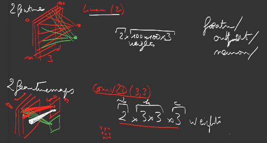
Last, a 1D-convolution can also be applied on matrices, where the first dimension is the length of the sequence and the second dimension is the dimensionality of the data, and modify the dimensionality of the data (number of channels):

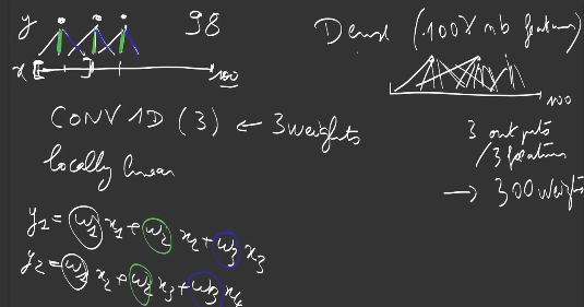
A 2D-convolution performs the same kind of computations on 2-dimensional inputs, with a 2-dimensional kernel \((k_1, k_2)\):

Contrary to Linear/Dense layers, where there is one weight (or 2, with the bias) per couple of input value and output value, which can be huge, a 1D-convolution has \(k \times d_{In} \times d_{Out}\) weights, a 2D-convolution has \(k_1 \times k_2 \times d_{In} \times d_{Out}\) weights if d is the number of output values:

One of the difficulty with convolutions is due to the fact the output featuremap shape depends on the kernel size and the stride:

since we want

To avoid that, it is possible to pad the input with 0 to create a larger input so that input and output featuremaps keep the same size. This simplifies the design of architectures:

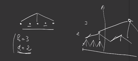
Last, convolutions can be dilated, in order to change the sampling scheme and the reach / the receptive field of the network. A dilated convolution of kernel 3 looks like a normal convolution of kernel 5 for which 2/5 of the kernel weights have been set to 0:

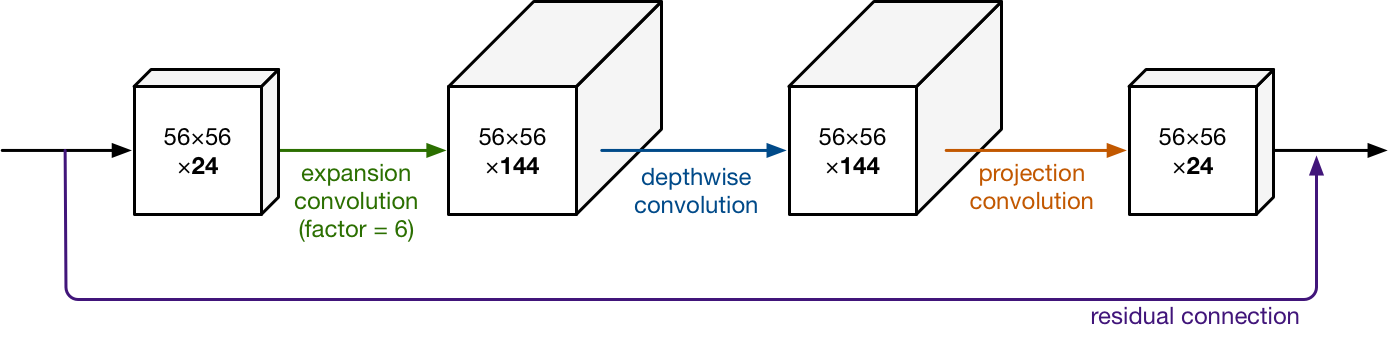
Note that a convolution of kernel 1 or (1x1) is called a pointwise convolution or projection convolution or expansion convolution, because it is used to change the dimensionality of the data (number of channels) without changing the length or the width and height of the data.

A convolution that applies convolutions on each channel without connections between channels is called a depthwise convolution. The combination of a depthwise convolution followed by projection convolution helps reduces the number of computations while maintaining the accuracy roughly.

Last, convolutions with kernel (k,1) or (1,k), processing only one dimension, either height or width, are called separable convolutions.

Pooling

Pooling operations are like Dense and Convolution Layers, but do not have weights. Instead, it performs a max or an averaging operation on the input.

There exists MaxPooling and AveragePooling, in 1D and 2D, as for convolutions:

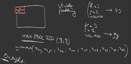
Usually used with a stride of 2, a MaxPooling of size 2 downsamples the input by 2, which helps summarizing the information towards the output, increases the invariance to small translations, while reducing the number of operations in the layers above.

There exists GlobalAveraging and GlobalMax, working the full input, as Dense layers do:

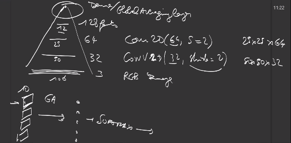
When a computer vision network transforms an image of shape (h,w,3) to an output of shape (H,W,C) where \(H \ll h\) and \(W \ll w\), then a global average pooling layer takes the average over all positions HxW : this helps build networks less sensitive to big translations of the object of interest in the image.

Normalization

Normalization layers are placed between other layers to ensure robustness of the trained neural network.

A first category of normalization layers aims at reducing internal covariance shift during training, i.e. that the statistics of the first layer below remains stable during training to help next layer better perform.

The mean and variance of the outputs are brought back to 0 and 1, by substraction and division, after which the normalization learn new scale and bias parameters.

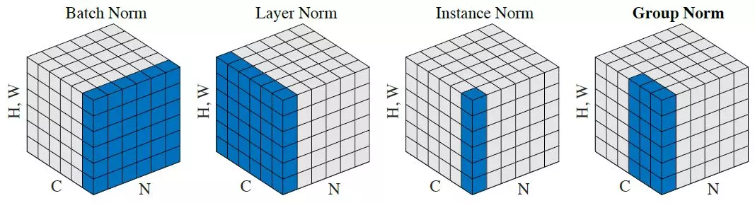
The statistics can be computed on different set:

• per channel but for all data in batch: batch normalization

• all channels but for one sample : layer normalization

• per channel and sample : instance normalization

• for a group of channels and per sample: group norm

Another type of normalization layers are dropout layers that drops some values by setting them to zero with a dropout probability in order to have the neural networks become more robust and regularized. In the stochastic depth training, some complete layers are dropped, a technique used in very deep networks such as ResNets and DenseNets.

Image classification

I’ll present some architectures of neural networks for computer vision. The primary trend was to build deeper networks with convolutional and maxpooling layers. Then, began the search for new efficient structures or modules to stack, rather than single layers. While the number of parameters and operations grew, another trend emerged to search for light-weight architectures for mobile devices and embedded applications.

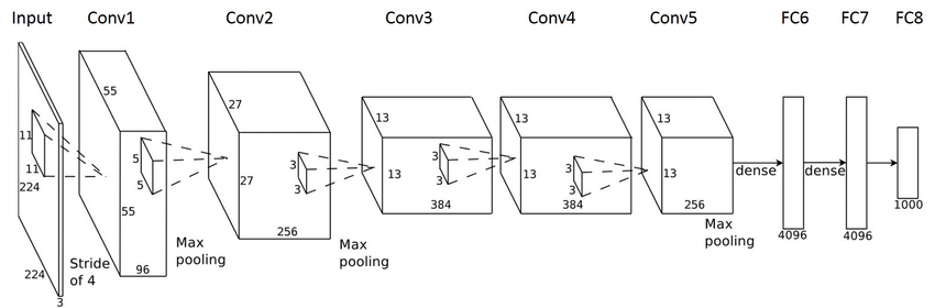
AlexNet (2012)

The network was made up of 5 convolution layers, max-pooling layers, dropout layers, and 3 fully connected layers (60 million parameters and 500,000 neurons).

It was the first neural network to outperform the state of the art image classification of that time and it won the 2012 ILSVRC (ImageNet Large-Scale Visual Recognition Challenge).

Main Points:

• Used ReLU (Rectified Linear Unit) for the nonlinearity functions (Found to decrease training time as ReLUs are several times faster than the conventional tanh function).

• Used data augmentation techniques that consisted of image translations, horizontal reflections, and patch extractions.

• Implemented dropout layers in order to combat the problem of overfitting to the training data.

• Trained the model using batch stochastic gradient descent, with specific values for momentum and weight decay.

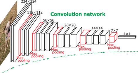
VGGNet (2014)

VGG neural architecture reduced the size of each layer but increased the overall depth of the network (up to 16 - 19 layers) and reinforced the idea that convolutional neural networks have to be deep in order to work well on visual data.

It finished at the first and the second places in the localisation and classification tasks respectively at 2014 ILSVRC.

Main Points

• The use of only 3x3 sized filters is quite different from AlexNet’s 11x11 filters in the first layer: the combination of two 3x3 conv layers has an effective receptive field of 5x5.

• It simulates a larger filter while decreasing in the number of parameters.

• As the spatial size of the input volumes at each layer decrease (result of the conv and pool layers), the depth of the volumes increase due to the increased number of filters as you go down the network.

• Interesting to notice that the number of filters doubles after each maxpool layer. This reinforces the idea of shrinking spatial dimensions, but growing depth.

GoogLeNet / Inception (2015)

GoogLeNet increases the depth of networks with much lower complexity: it is one of the first models that introduced the idea that CNN layers didn’t always have to be stacked up sequentially and creating smaller networks or “modules” :

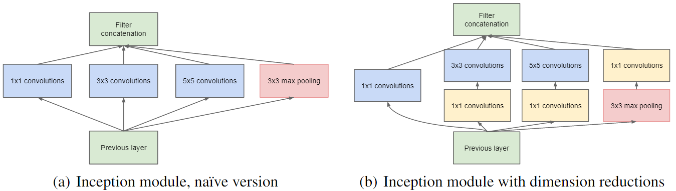
that could be repeated inside the network:

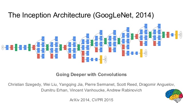
GoogLeNet is a 22 layer CNN and was the winner of ILSVRC 2014

Main Points

• Used 9 Inception modules in the whole architecture, with over 100 layers in total!

• No use of fully connected layers : it use an average pool instead, to go from a 7x7x1024 volume to a 1x1x1024 volume. This saves a huge number of parameters.

• Uses 12x fewer parameters than AlexNet.

• During testing, multiple crops of the same image are fed into the network, and the softmax probabilities are averaged to give the final prediction.

• There are updated versions of the Inception module.

This work was a first step towards the development of grouped convolutions in the future.

ResNet (2015)

ResNet utilizes efficient bottleneck structures and learns them as residual functions with reference to the layer inputs, instead of learning unreferenced functions :

where R is a residual to learn.

Residuals are stacks of convolution.

That structure is then sequentially stacked several tenth of time (or more).

The winner of the classification task of ILSVRC 2015 is a ResNet network.

Main Points

• On the ImageNet dataset residual nets of a depth of up to 152 layers were used being 8x deeper than VGG nets while still having lower complexity.

• Residual networks are easier to optimize than traditional networks and can gain accuracy from considerably increased depth. In fact, they do not suffer from the vanishing gradients when the depth is too important.

• Residual networks have a natural limit : a 1202-layer network was trained but got a lower test accuracy, presumably due to overfitting.

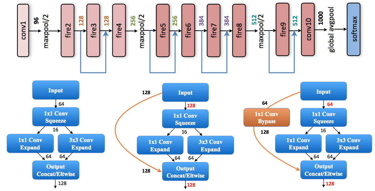
SqueezeNet (2016)

Up to this point, research focused on improving the accuracy of neural networks, the SqueezeNet team took the path of designing smaller models while maintaining the accuracy unchanged.

It resulted into SqueezeNet, which is a convolutional neural network architecture that has 50 times fewer parameters than AlexNet while maintaining its accuracy on ImageNet.

3 main strategies are used while designing that new architecture:

• Replace the majority of 3x3 filters with 1x1 filters (to fit within a budget of a certain number of convolution filters).

• Decrease the number of input channels to 3x3 filters, using dedicated filters named squeeze layers.

• Downsample late in the network so that convolution layers have large activation maps.

The first 2 strategies are about judiciously decreasing the quantity of parameters in a CNN while attempting to preserve accuracy.

The last one is about maximizing accuracy on a limited budget of parameters.

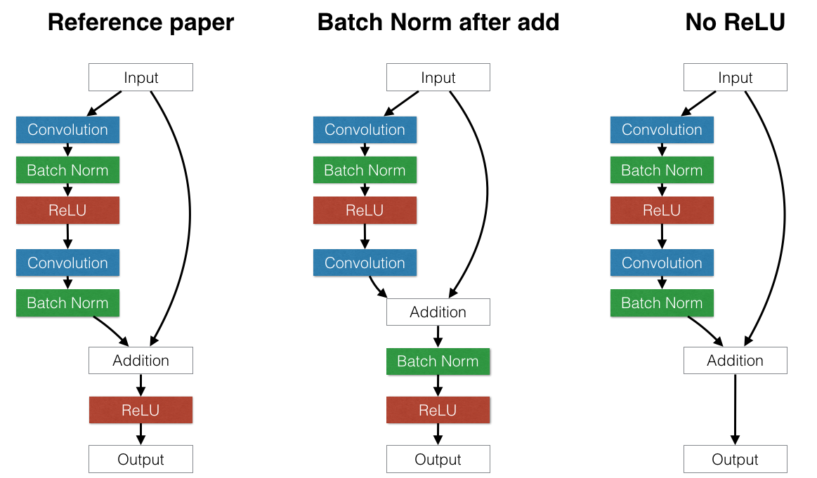
PreActResNet (2016)

PreActResNet stands for Pre-Activation Residuel Net and is an evolution of ResNet described above.

The residual unit structure is changed from (a) to (b) (BN: Batch Normalization) :

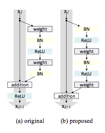
The activation functions ReLU and BN are now seen as “pre-activation” of the weight layers, in contrast to conventional view of “post-activation” of the weighted output.

This changes allowed to increase further the depth of the network while improving its accuracy on ImageNet for instance.

DenseNet (2016)

DenseNet is a network architecture where each layer is directly connected to every other layer in a feed-forward fashion (within each dense block). For each layer:

• the feature maps of all preceding layers are treated as separate inputs,

• its own feature maps are passed on as inputs to all subsequent layers.

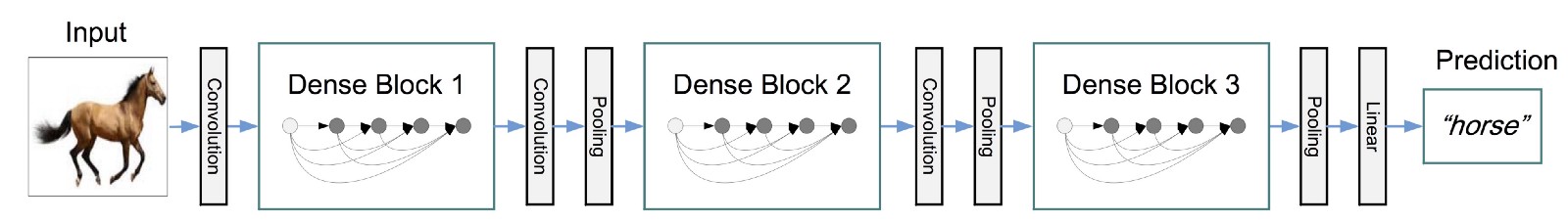
This connectivity pattern yields on CIFAR10/100 accuracies as good as its predecessors (with or without data augmentation) and SVHN. On the large scale ILSVRC 2012 (ImageNet) dataset, DenseNet achieves a similar accuracy as ResNet, but using less than half the amount of parameters and roughly half the number of FLOPs.

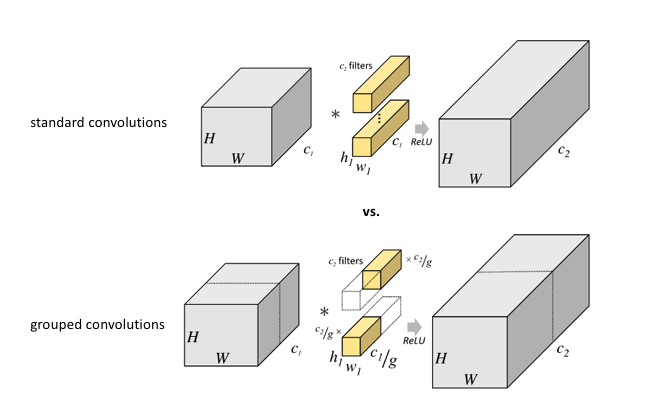
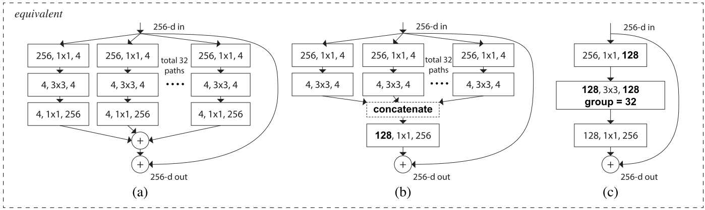
ResNeXt (2016)

The neural network architecture ResNeXt is based upon 2 strategies :

• stacking building blocks of the same shape (strategy inherited from VGG and ResNet)

• the “split-transform-merge” strategy that is derived from the Inception models and all its variations (split the input, transform it, merge the transformed signal with the original input).

That design introduces group convolutions and exposes a new dimension, called “cardinality” (the size of the set of parallel transformations), as an essential factor in addition to the dimensions of depth and width.

It is empirically observed that :

• when keeping the complexity constant, increasing cardinality improves classification accuracy.

• increasing cardinality is more effective than going deeper or wider when we increase the capacity.

ResNeXt finished at the second place in the classification task at 2016 ILSVRC.

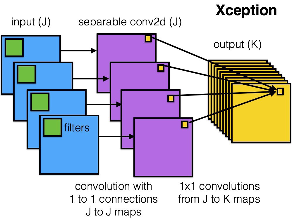
Xception (2016)

Xception introduces depthwise separable convolutions that generalize the concept of separable convolutions in Inception.

DPN (2017)

DPN is a family of convolutional neural networks that intends to efficiently merge residual networks and densely connected networks to get the benefits of both architecture:

• residual networks implicitly reuse features, but it is not good at exploring new ones,

• densely connected networks keep exploring new features but suffers from higher redundancy.

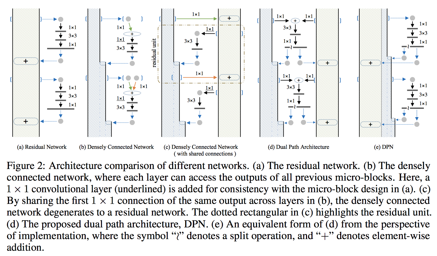
Consequently, DPN (Dual Path Network) contains 2 path :

• a residual alike path (green path, similar to the identity function),

• a densely connected alike path (blue path, similar to a dense connection within each dense block).

NASNet (2017)

NASNet learns to architect a the neural network itself, by the Neural Architecture Search (NAS) framework, which uses a reinforcement learning search method to optimize architecture configuration.

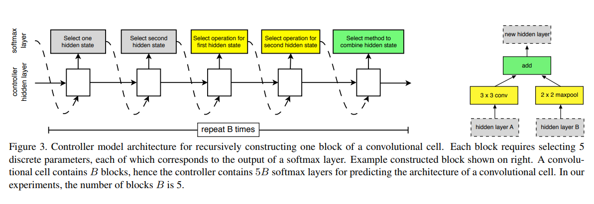
Each network proposed by the RI network is further trained and its accuracy is our reward. To keep the computational effort affordable, the training is performed on a subset of the complete dataset.

The key principle of this model is the design of a new search space (named the “NASNet search space”) which enables transferability from the smallest dataset to the complete one.

Two new modules have been found to achieve state-of-the-art accuracy.

SENet (2017)

Typical convolutional neural networks builds a description of its input image by progressively capturing patterns in each of its layers. For each of them, a set of filters are learned to express local spatial connectivity patterns from its input channels. Convolutional filters captures informative combinations by fusing spatial and channel-wise information together within local receptive fields.

SENet (Squeeze-and-Excitation Networks) focuses on the relation between channels and recalibrates at transformation step its features so that informative features are emphazised and less useful ones suppressed (independently of their spatial location).

To do so, SENet uses a new architectural unit that consists of 2 steps :

• First, squeeze the block input (typically the output of any other convolutional layer) to create a global information using global average pooling,

• Then, “excite” the most informative features using adaptive recalibration.

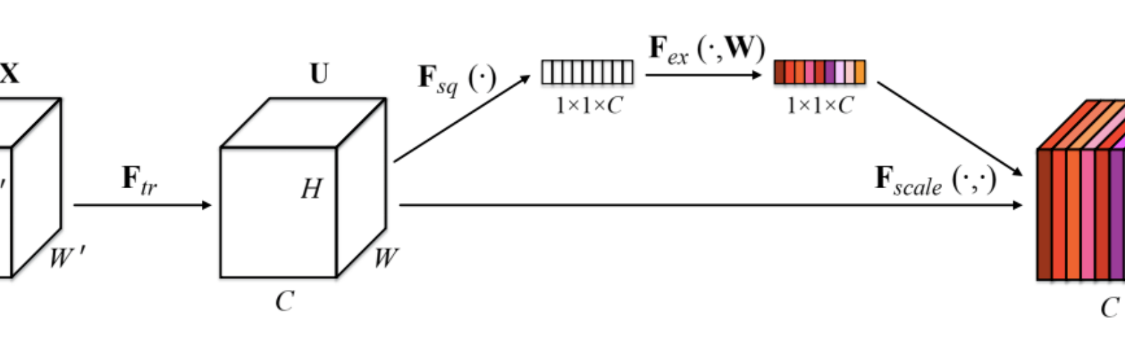
The adaptative recalibration is done as follows :

• reduce the dimension of its input using a fully connected layer (noted FC below),

• go through a non-linearity function (ReLU function),

• restore the dimension of its data using another fully connected layer,

• use sigmoid function to transform each output into a scale parameter between 0 and 1,

• linearly rescale each original input of the SE unit according to the scale parameters.

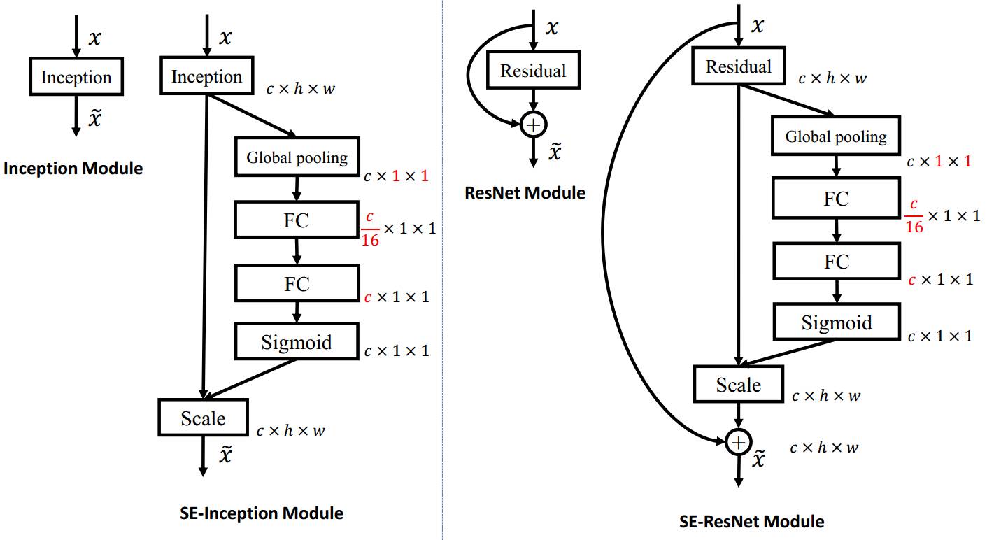
The winner of the classification task of ILSVRC 2017 is a modified ResNeXt integrating SE blocks.

MobileNets and Mobilenetv2

There has been also recently some effort to adapt neural networks to less powerful architecture such as mobile devices, leading to the creation of a class of networks named MobileNet, with a new module optimized for mobility:

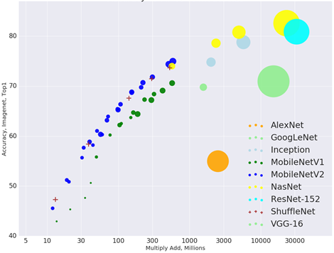
The diagram below illustrates that accepting a (slightly) lower accuracy than the state of the art, it is possible to create networks much less demanding in terms of resources (note that the multiply/add axis is on a logarithmic scale).

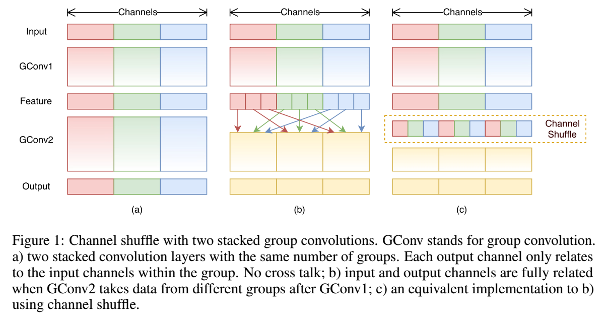
ShuffleNet

ShuffleNet goes one step further:

• by replacing the pointwise group convolutions that become the main cost, with pointwise group convolutions

• shuffling the output of group convolutions so that information can flow from each to group to each group of the next group convolution:

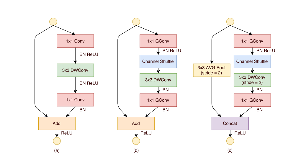
While (a) is the bottleneck unit from Xception, grouping the features in the first pointwise convolution requires to shuffle the data to the next (b). When the module is asked to reduce the featuremap size, the depthwise convolution has a stride 2, an average pooling of stride 2 is applied to the shortcut connection and the output channels of both paths are concatenate rather than added, in order to augment the channel dimension (c).

Group convolutions reduces the budget so featuremaps can be extended with more channels, bringing a better accuracy in smaller models.

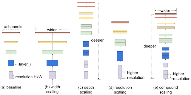
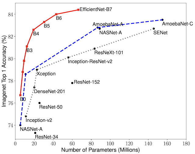
EfficientNet and Compound scaling

Since then, increasing width (more filters per layer) or depth (more layers) of a neural network increased its capacity, and its accuracy, up to a certain size. Working with inputs of higher resolution was also a way to improve accuracy, despite a strong increase in computation cost as for width. Then, it has been noticed that increasing these three dimensions (depth, width and resolution) together rather than separately lead to better accuracy. They propose a method to scale architectures : given a baseline network, you search (with grid search) for hyperparameters \(\alpha^\phi\), \(\beta^\phi\) and \(\gamma^\phi\) to scale depth, width and resolution so that it doubles the number of parameters in the network, i.e. \(\alpha \cdot \beta^2 \cdot \gamma^2 = 2\) and leads to the best accuracy. Then, you simply increase \(\phi\) to scale the network to a higher factor than 2. With this method, they successfully increased the size of baselines ResNet-50, MobileNetv1 and MobileNetv2 towards better accuracy than with only one dimension.

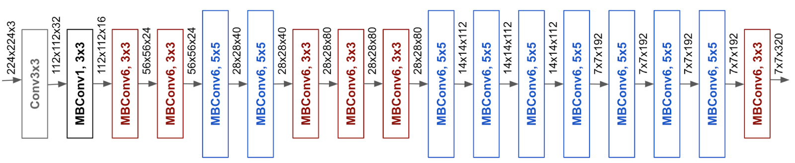
Under their method of compound scaling, finding the best networks can be summarized by the efficiency of the baseline network, that they can search at lower computational cost or at a target computational cost T. They released the EfficientNet architecture, found with the neural architecture search method on an objective trading accuracy with FLOPS:

The mobile inverted bottleneck MBConv (Sandler et al., 2018; Tan et al., 2019) is the main building block:

The resulting accuracy :

Exercise: use a Pytorch model to predict the class of an image.

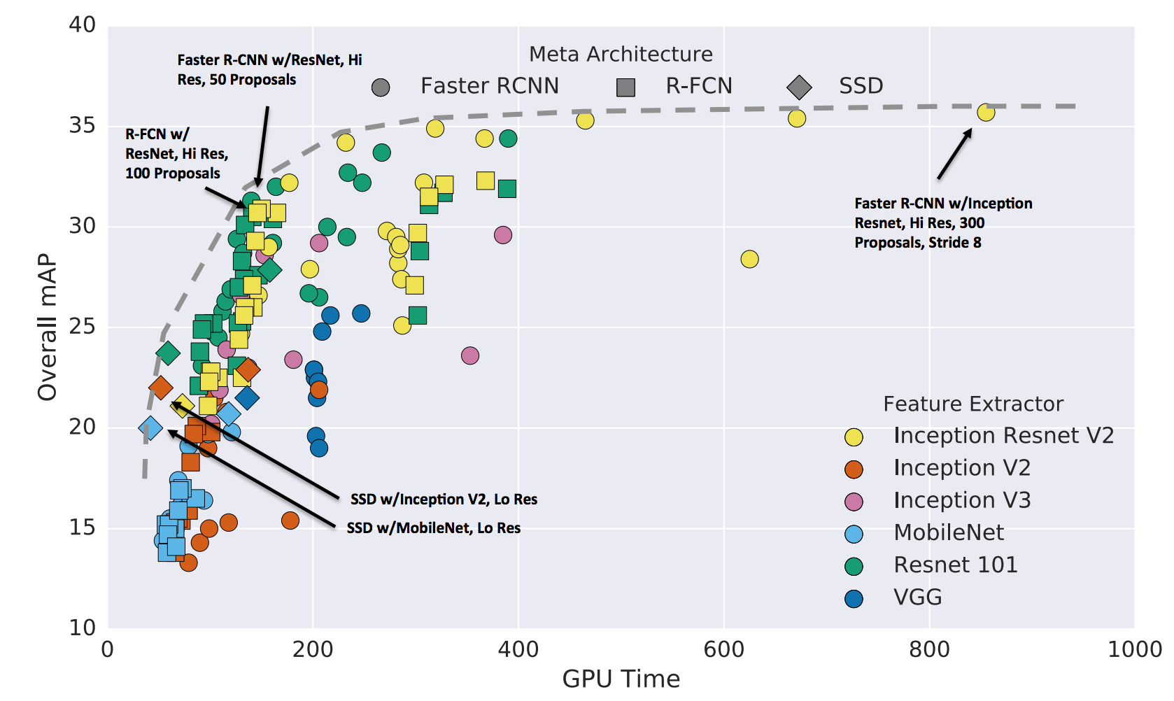
Object detection

For object detection, the first layers of the Image classification networks serve as a basis as “features”, on top of which new neural network parts are learned, using different techniques: Faster-RCNN, R-FCN, SSD, …. The pretrained layers of Image classification networks have learned a “representation” of the data on high volume of images that helps train object detection neural architectures on specialized datasets. Below is a diagram presenting differente object detection techniques with different features. When the feature network is more efficient for image classification, results in object detection are also better.

Segmentation

Audio

Well done!

Next course ! natural language and deep learning