Course 0: Why targets 0 and 1 in machine learning ?
Here is my course of deep learning in 5 days only!
First, we’ll begin by the basic concepts in this article, because main deep learning concepts come from datascience. This is a great article for an experienced datascientist also.
I hope you’ll get some feelings about deep learning you cannot get from reading else where.
First, let’s recap the basics of machine learning.
Loss functions
When we fit a model, we use loss functions, or cost functions, or objective functions. The main purpose of machine learning is to be able to predict given data. Let’s say predict the \(y\) given some observations, let’s say the \(x\), through a function:
\[f : x \rightarrow y\]Usually, f is called a model and is parametrized, let’s say by a list of parameters \(\theta\)
\[f = f_\theta\]and the goal of machine learning is to find the best parameters.
In supervised learning we know the real value we want to predict \(\tilde{y}\), for example the class of the object we want to predict, what we call the ground truth or the target.
We want to be able to measure the difference between what we are predicted with the model \(f\) and what it should predict. For that, there are some cost functions, depending on the problem you want to address, to measure how far our predictions are from their targets.
\[L(y, \tilde{y})\]In order to minimize the cost, we prefer differentiable functions which have simpler optimization algorithms.
The two most important loss functions are:
-
Mean Squared Error (MSE), usually used for regression: \(\sum_i (y_i - \tilde{y_i})^2\)
-
Cross Entropy for probabilities, in particular for classification where the model predicts the probability of the observed object x for each class or “label”:
Coming from the theory of information, cross-entropy measures the distance between two probabilities by :
\[\text{CrossEntropy}(p, \tilde{p}) = - \sum_c \tilde{p}_c \log(p_c)\]which can be defined as the expected log-likelihood of the predicted label under the true label distribution, and we want this cost to be the lowest possible (minimization).
Note that a loss function always outputs a scalar value. This scalar value is a measure of fit of the model with the real value. Since a loss function outputs a scalar, the shape of its Jacobian with respect to an input is the same as the shape of the input, for example for an input of rank 4:
\[\nabla f = \Big[ \frac{\partial f}{\partial I_{a,b,c,d}} \Big]_{a,b,c,d}\]In conclusion of this section, the goal of machine learning is to have a function fit with the real world; and to have this function fit well, we use a loss function to measure how to reduce this distance.
Exercise: discover many more loss functions with my full article about loss functions.
Cross entropy in practice
Two problems arise: first, most mathematical functions do not output a probability vector which values sum to 1. Second, how do I evaluate the true distribution \(\tilde{p}\) ?
Normalizing model outputs
Usually, transforming any model output into a probability that sums to 1 is usually performed thanks to a softmax function set on top of the model outputs :
\[x \xrightarrow{f} o = f(x) = \{o_c\}_c \xrightarrow{softmax} \{p_c\}_c\]The softmax normalization function is defined by:
\[\text{Softmax}(o) = \Big\{ \frac{ e^{o_i} }{ \sum_c e^{o_c}} \Big\}_i\]Note that for the softmax to predict probability for C classes, it requires the output \(o = f(x)\) to be C-dimensional. \(\{o_c\}_c\) are called the logits.
Softmax is the equivalent of the sigmoid() in binary classification:
in the multi-class case. If you do not remember which one between the softmax and the sigmoid has a negative sign in the exponant, ie \(e^x\) or \(e^{-x}\), remember that Softmax and Sigmoid are both monotonic functions.
Estimating the true distribution
Cross entropy is usually mentioned without explanations.
In fact, to understand cross-entropy, you need to rewrite its theoretical definition (1):
\[\text{CrossEntropy} = - \sum_c \tilde{p_c} \log p_c = - \mathbb{E} \Big( \log p_c \Big)\]because \(\tilde{p_c}\) is the true label distribution, so cross entropy is the expectation of the negative log-probability predicted by the model under the true distribution.
Then, we use the formula for the empirical estimation of the expectation:
\[\text{CrossEntropy} \approx - \frac{1}{N} \sum_{x \sim D} \log p_{\hat{c}(x)}(x) = \text{EmpiricalCrossEntropy}(p)\]where D is the real sample distribution, N is the number of samples on which the cross entropy is estimated (\(N \gg 1\)) and \(\hat{c}(x)\) is the true class of x.
When we compute the cross-entropy, we set an empirical cross-entropy for one sample (N=1) to
\[\text{CrossEntropy} \approx - \log p_\hat{c}(x)\]so that when we average the individual losses over more samples for stability, we find back to the desired empirical estimation:
\[\frac{1}{N} \sum_{x \sim D} L(x) = - \frac{1}{N} \sum_{x \sim D} \log p_{\hat{c}(x)}(x) = \text{EmpiricalCrossEntropy}(p)\]In the future, we adopt the following formulation for a single sample:
\[\text{CrossEntropy}(p) = - \log p_\hat{c}(x)\]which is equivalent to setting the \(\tilde{p}\) probability in the theoretical cross-entropy definition (1) with:
\[\tilde{p}_c(x) = \begin{cases} 1, & \text{if } c = \hat{c}(x), \\ 0, & \text{otherwise}. \end{cases}\]which we will write \(\tilde{p}_c(x) = \delta(c,\hat{c})\). That is why the target for the predicted probability for the true class is 1.
\(\tilde{p}\) is a vector of zero values except for the true class, where it has a one: we name \(\tilde{p}\) the one-hot encoding.
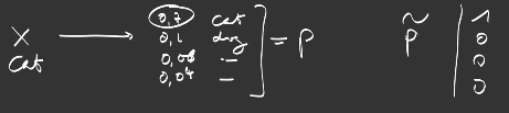
In conclusion, for the case of classification, we compute the cross-entropy with values that are either 0 or 1 at the sample level for the “true” probability: x being the image of a cat, we want the model output \(\{p_c\}_c\) to fit the empirical class probability \(\{\tilde{p}_c\}_c\) at the sample level, that we set to \(\tilde{p}_\hat{c} = 1\) for the real object class \(\hat{c}\) “cat” and \(\tilde{p}_c = 0\) for all other classes \(c \neq \hat{c}\): then at the dataset level, averaging these values lead to the empirical estimates of the true probabilities we are used to.
The Gradient Descent
To minimize the cost function, the most used technique is the Gradient Descent.
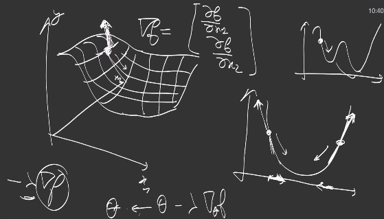
It consists in following the gradient to descend to the minima:
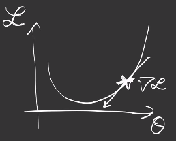
In other words, we follow the negative slope of the mountain to find the bottom/lowest position of the valley. In order to avoid a local minima, initialization (the choice of initial values for the parameters, where to start the descent from) is very important, and multiple runs can also help find the best solution.
It is an iterative process in which the update rule simply consists in:
\[\theta_{t+1} = \theta_{t} - \lambda \nabla_\theta \text{cost}\]where our cost is defined as a result of the previous section
\[\text{cost}_\theta (x, \tilde{p}) = \text{CrossEntropy} ( \text{Softmax}( f_\theta (x) ) , \tilde{p})\]We call \(\tilde{p}\) the target (in fact the target distribution). We usually omit the fact the cost is a function of the input, the target and the model parameters and write it directly as “cost”. We can also write with the composition symbol:
\[\text{cost} = \text{CrossEntropy} ( \cdot, \tilde{p}) \circ \text{Softmax} \circ f_\theta\]
An update rule is how to update the parameters of the model to minimize the cost function.
Since the cost is a scalar, the Jacobian has the same shape as the parameters, and gives a derivative value with respect to every parameter, telling us how to update it.
\(\lambda\) is the learning rate and has to be set carefully: Effect of various learning rates on convergence (Img Credit: cs231n)

This simple method is named SGD, after Stochastic Gradient Descent. There are many improvements around this simple rule: ADAM, ADADELTA, RMS Prop, … All of them are using the first order only. Some are adaptive, such as ADAM or ADADELTA, where the learning rate is adapted to each parameter automatically.
There exists some second order optimization methods also but they are not very common in practice.
Conclusion: When we have the loss function, the goal is to minimize it. For this, we have a very simple update rule which is the gradient descent.
Backpropagation
Computing the gradients to use in the SGD update rule is known as backpropagation.
The reason for this name is the chaining rule in computing gradients of function compositions.
First, adding the softmax and cross-entropy to the model outputs is a composition of 3 functions:
\[\text{cost} = \text{CrossEntropy} \circ \text{Softmax} \circ f_\theta\]where the composition means
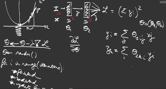
\[\text{cost}(x) = \text{CrossEntropy} (\text{Softmax} ( f_\theta(x) ) )\]But models are also composed of multiple functions, for example let us consider a model composed of 2 dense layers:
\[\text{cost} = \text{CrossEntropy} \circ \text{Softmax} \circ \text{Dense}_{\theta_2}^2 \circ \text{ReLu} \circ \text{Dense}_{\theta_1}^1\] \[\text{cost}(x) = \text{CrossEntropy} (\text{Softmax} (\text{Dense}_{\theta_2}^2 ( \text{ReLu} ( \text{Dense}_{\theta_1}^1 (x) ) ) ) )\]This model is called perceptron and the output of the first Dense layer is a hidden representation of the data, while the second layer is used to reduce the number of outputs to the number of classes, to predict class probabilities with a softmax normalization:
Without a ReLu activation in the middle, the two Dense layers would be mathematically equivalent to only 1 Dense layer.
The model has two sets of parameters:
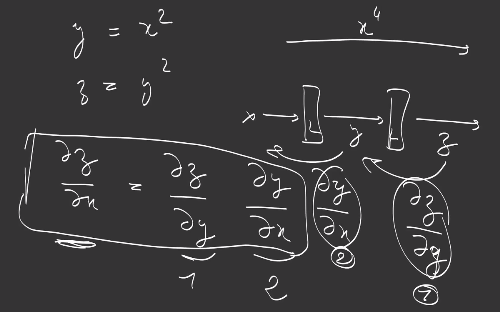
\[\theta = [ \theta_1, \theta_2 ]\]The chaining rule is a rule for gradient computation of the composition of two functions f and g:
\[\frac{ \partial }{ \partial x_i} (f \circ g )_k = \sum_c \frac{\partial f_k}{\partial g_c} \cdot \frac{\partial g_c}{\partial x_i}\]which is a simple matrix multiplication
\[\nabla (f \circ g) = \nabla f \times \nabla g\]if
\[\nabla f = \Big\{ \frac{\partial g_i}{\partial x_j} \Big\}_{i,j}\]What does that mean for deep learning and gradient descent ? In fact, for each layer, to follow the negative slope, we need to compute
\[\nabla_{\theta_{\text{Layer}}} \text{cost}\]to update each layer’s parameters \(\theta_{\text{Layer}}\).
So, let’s consider a two layer network composed of g and f. The functions g and f have to be considered as functions of both inputs and parameters:
\[g(x) = g_{\theta_g} (x) = g(x,\theta_g)\] \[f(y) = f_{\theta_f} (y) = f(y,\theta_f)\]And the composition becomes
\[(f \circ g)(x) = f_{\theta_f} ( g(x,\theta_g), \theta_f)\]It is possible to compute the derivatives of g and f with respect to, either the parameters, or the inputs, which we’ll differentiate in notation the following way:
\[\nabla_{\theta_g} g = \Big\{ \frac{\partial g_i}{\partial {\theta_g}_j } \Big\}_{i,j}\] \[\nabla_I g = \Big\{ \frac{\partial g_i}{\partial x_j} \Big\}_{i,j}\]To update the parameters of g, we need to compute the derivative of the cost with respect to the parameters of g, that is :
\[\nabla_{\theta_g} (f \circ g_{\theta_g}) = \nabla_I f \times \nabla_{\theta_g} g\]all other parameters (\(\theta_f\)) and inputs (x) being constant.
For example, for the layer \(\text{Dense}^2\),
\[x \xrightarrow{ \text{Dense}^1 } \xrightarrow{ \text{ReLu} } y \xrightarrow{ \text{Dense}^2 } \xrightarrow{ \text{Softmax}} \xrightarrow{ \text{CrossEntropy} } \text{cost}\]the gradient is given by
\[\nabla_{\theta_2} \text{cost} = \nabla_{\theta_2} \Big( \text{CrossEntropy} \circ \text{Softmax} \circ \text{Dense}^2 \Big)\] \[= \Big(\nabla_I \text{CrossEntropy} \times \nabla_I \text{Softmax}\Big) \times \nabla_{\theta_2} \text{Dense}^2\]and for the layer \(\text{Dense}^1\),
\[\nabla_{\theta_1} \text{cost} = \Big(\nabla_I \text{CrossEntropy} \times \nabla_I \text{Softmax}\Big) \times \nabla_I \text{Dense}^2 \times \nabla_I \text{ReLu} \times \nabla_{\theta_1} \text{Dense}^1\]We see that \(\Big(\nabla_I \text{CrossEntropy} \times \nabla_I \text{Softmax}\Big)\) is common to the computation of \(\nabla_{\theta_1} \text{cost}\) and \(\nabla_{\theta_2} \text{cost}\), and it is possible to compute them once.
So, to reduce the number of matrix mulplications, it is better to compute the gradients from the top layer to the bottom layer and reuse previous computations of matrix multiplication from earlier layers.
In conclusion, gradient computation with respect to each layer’s parameters is performed via matrix multiplications of gradients of the layers above, so it is more efficient to begin to compute gradients from the top layers, a process we call retropropagation or backpropagation.
Cross Entropy with Softmax
Let’s come back to the global view: an observation X, a model f depending on parameters \(\theta\), a softmax to normalize the model’s output, and last, our cross entropy outputting a final scalar, measuring the distance between the prediction and the expected value:
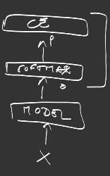
The cross entropy is working very well with the softmax function and is usually implemented as one layer, for numerical efficiency.
Let us see why and study the combination of softmax and cross entropy
\[o = f(x) = \{o_c\}_c \xrightarrow{ \text{Softmax}} \xrightarrow{ \text{CrossEntropy} } \text{cost}\]Mathematically,
\[\text{cost} = - \log(p_\hat{c}) = - \log \Big( \frac{ e^{o_\hat{c}} }{ \sum_c e^{o_i}} \Big)\] \[= - \log e^{o_\hat{c}} + \log \sum_c e^{o_i}\] \[= - o_\hat{c} + \log \sum_c e^{-o_i}\]Let’s take the derivative with respect to the model output (before softmax normalization):
\[\frac{\partial \text{cost}}{\partial o_c} = - \delta_{c,\hat{c}} + \frac{ e^{o_i} }{\sum_c e^{o_i}}\] \[= - \delta_{c,\hat{c}} + p_c\]which is very easy to compute and can simply be rewritten:
\[\nabla_o \text{cost} = p - \tilde{p}\]Note that the gradient is between -1 and 1: for a negative class (\(\tilde{p} = 0\)), the derivative is positive, and the higher the prediction has been positive, the higher the derivative will be; for a positive class, the derivative will always be negative, and the lower the prediction to be positive, the lower the derivative will be.
Since Softmax is monotonic, Softmax output computation is not required for inference, the highest logit corresponds to the highest probability… except if you need the probability to estimate the confidence of the predicted class.
Conclusion: it is easier to backprogate gradients computed on Softmax+CrossEntropy together rather than backpropagate separately each : the derivative of the Softmax+CrossEntropy with respect to the output of the model for the right class, let’s say the “cat” class, will be 0.8 - 1 = - 0.2, if the model has predicted a probability of 0.8 for this class, and the update will follow the negative slope to encourage to increase the prediction ; the derivative of the Softmax+CrossEntropy with respect to an output for a different class will be 0.4 is it has predicted a probability of 0.4, encouraging the model to decrease this value.
Exercise: Compute the derivative of Sigmoid+BinaryCrossEntropy combined.
Exercise: Compute the derivative of Sigmoid+MSE combined.
Example with a Dense layer
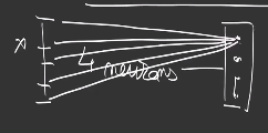
Let’s take, as model, a very simple one with only one Dense layer with 2 filters in one dimension and an input of dimension 2:
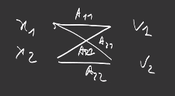
This is the smallest model we can ever imagine. Such a layer produces a vector of 2 scalars:
\[f_\theta : \{x_j\} \rightarrow \Big\{ o_i = \sum_j \theta_{i,j} x_j + b_i \Big\}_i\]Please keep in mind that it is not possible to descend the gradient directly on this output because it is composed of two scalars. We need a loss function, that returns a scalar, and tells us how to combine these two outputs. For example, the Softmax+CrossEntropy we have seen previously:
\[L :o \rightarrow \text{CrossEntropy}(\text{Softmax}(o))\]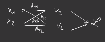
Now we can retropropagate the gradients. Since we are in the case of 2 outputs, we call this problem a binary classification problem, let’s say: cats and dogs.
Let us compute the derivatives of the dense layer:
\[\frac{\partial o_i}{\partial \theta_{k,j}} = \begin{cases} x_j, & \text{if } k = i, \\ 0, & \text{otherwise}. \end{cases}\]so
\[\frac{\partial}{\partial \theta_{i,j}} ( L \circ f_\theta )= \sum_c \frac{\partial L}{\partial o_c} \cdot \frac{\partial o_c}{\partial \theta_{i,j}} = \frac{\partial L}{\partial o_i} \cdot \frac{\partial o_i}{\partial \theta_{i,j}} = ( \delta_{ i, \hat{c}} - L(o_i)) \cdot x_j\]A Dense layer with 4 outputs:
Generalize beyond cross entropy
Re-weighting probabilities
Cross-entropy is built upon the probability of the label:
\[\text{CrossEntropy} = - \sum_c \tilde{p_c} \log p_c\]In our section on practical cross-entropy, we have considered that we knew the true label with certainty, that the goal to achieve was maximize the objective under the real distribution of labels, even if they are unbalanced in the dataset, leading to strong bias. In practice, we can go one step further, rebalancing these probability as Bayes rules would suggest, or integrate the notion of incertainty in the groundtruth label, to reduce the influence of noise. Here are a few techniques we can use in practice. It is still possible:
- to rebalance the dataset with \(\alpha_{c}\) the inverse class frequency :
This could also be performed by replacing the current sampling schema (\(\tilde{p}\)), by sampling uniformly the class first, then a sample belonging to this class.
- to train a model with smoother values than 0 and 1 for negatives and positives, for example 0.1 or 0.9, which will help achieve better performances. This technique of label smoothing or soft labels enables in particular to re-introduce the outputs for the negative classes so that it will preserve a symmetry between the negative and positive labels:
This technique reduces the confidence in the targets, and the network overfitting. It discourages too high differences between the logits for the true class and for the other classes.
It is also possible to regularize with label smoothing, by drawing with probability \(\epsilon\) a class among C classes uniformly:
\[\tilde{p}' (c) =(1-\epsilon) \delta_{c,\hat{c}} + \frac{\epsilon}{C}\] \[\text{CrossEntropy'}(p, \tilde{p}) = (1-\epsilon) \text{CrossEntropy}(p, \tilde{p}) + \epsilon \text{CrossEntropy}(p, \text{uniform})\]-
to use smoother values than 0 and 1 when the labels in the groundtruth are less certain,
-
to focus more on wrongly classified examples
as in the Focal Loss for object detection where background negatives are too numerous and tend to take over the positives. This technique replaces hard negative mining.
Reinforcement
That is where the magic happens ;-)
As you might have understood, the cross entropy comes from the theory of information, but the definition of the probabilities and their weighting scheme can be adapted to the problem we want to solve. That is where we leave theory for practice.
Still, there is a very important theoretical generalization of cross-entropy through reinforcement learning which is very easy to understand.
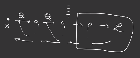
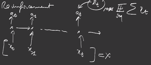
In reinforcement, given an observation \(x_t\) at a certain timestep, you’re going to perform an action, for example driving car, going right, left, or straight, or in a game, using some keyboard commands. Then the environment is modified and you’ll need to decide of the next action… and sometimes you get a reward \(r_t\), a feedback from the environment, good news or bad news, gain some points… In the case of reinforcement learning, we do not have any labels as targets or groundtruth. We just want to get the best reward :
\[R = \mathbb{E}_{\text{seq}} \sum_{t} r_t\]over all possible sequence of actions.
The probability of a sequence is
\[p({a_0, a_1, ..., a_T}) = p (a_0 | x_0) p( a_1 | a_0, x_0, x_1)... = \prod_{t=0}^T p(a_t | a_0, x_0, ... x_T)\]so R can be written
\[R = \sum_{a_0, a_1, ..., a_T} \big( \prod_{t=0}^T p(a_t | a_0, x_0, ... x_T) \big) (\sum_{t=0}^T r_t)\] \[= \mathbb{E}_{a_0 \sim p(\cdot |x_0)} \mathbb{E}_{a_1 \sim p(\cdot | a_0, x_0, x_1)} ... \mathbb{E}_{a_T \sim p(\cdot | a_0, x_0, ... x_T)} \sum_{t=0}^T r_t\]When my actions are parametrized by a model \(p = f_\theta\), the whole problem becomes parametrized by \(\theta\) and it is possible to find the \(\theta\) that maximizes the reward by following the gradient of the expected reward:
\[R(\theta) = \mathbb{E}_{\text{seq} \sim p_\theta} \sum_{t=0}^T r_t = \sum_{\text{seq}} p_\theta(\text{seq}) \sum_{t=0}^T r_t\]In order to maximize the expected reward \(J(\theta)\), we compute the derivative:
\[\nabla_\theta R = \sum_{\text{seq}} \frac{\partial p_\theta(\text{seq})}{\partial \theta} (\sum_{t=0}^T r_t) = \sum_{\text{seq}} p_\theta(\text{seq}) \frac{\partial \log p_\theta(\text{seq})}{\partial \theta} (\sum_{t=0}^T r_t) = \mathbb{E}_{\text{seq}} \frac{\partial \log p_\theta(\text{seq})}{\partial \theta} (\sum_{t=0}^T r_t)\]because \(\frac{\partial f}{\partial \theta} = f \times \frac{1}{f} \frac{\partial f}{\partial \theta} = f \times \frac{\partial \log f}{\partial \theta}\)
which looks exactly the same as the derivative of the cross entropy:
\[\text{CE} = \sum_c \log(p_c) \tilde{p_c}\] \[\frac{\partial \text{CE}}{\partial \theta} = \sum_c \frac{\partial \log(p_c)}{\partial \theta} \tilde{p_c}\]except that you replace the expected reward in place of the true label probability:
\[\log p_\theta(\text{seq}) = \log \prod_{t=0}^T p_\theta(a_t | a_0, x_0, ... x_t)\] \[= \sum_{t=0}^T \log p_\theta (a_t| a_0, x_0, ... x_t)\] \[\frac{\partial \log p_\theta(\text{seq}) }{ \partial \theta } = \sum_{t=0}^T \frac{\partial \log p_\theta (a_t| a_0, x_0, ... x_t)}{\partial \theta}\] \[\nabla_\theta R = \mathbb{E}_{\text{seq}} ( \sum_{t=0}^T \frac{\partial \log p_\theta (a_t| a_0, x_0, ... x_t)}{\partial \theta} ) \times ( \sum_{t=0}^T r_t )\]In conclusion, in place of the 1 and 0 of the classification case, reinforcement learning proposes to use the global reward R as target label for each timestep that led to this reward, considering each time step as individual samples.
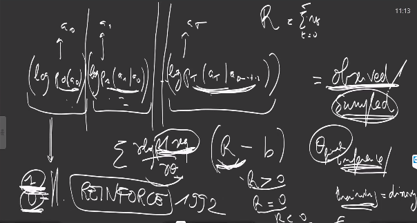
A fantastic demonstration [Williams, 1992] of re-weighting the cross-entropy, where the eligibility of each parameter to the gradient is multiplied by the reward or the progress in the goal we want to achieve.
Classical cross-entropy definition can be seen as a specific case of this more global theorization.
Well done!
Now let’s go to next course: Course 1: programming deep learning!